langchain enables agentic code to invoke one or more agents
from langchain.agents import load_tools
from langchain.agents import initialize_agent
from langchain.llms import OpenAI
llm = OpenAI(temperature=0)
tools = load_tools(["serpapi", "llm-math"], llm=llm)
agent = initialize_agent(tools, llm, agent="zero-shot-react-description", verbose=True)
agent.run("how can one fine-tune a generative ai llm model ?")
here’s the output, showing it “thinking” through the steps to answer the question posed.
$ python langchain-test.py


> Entering new AgentExecutor chain...
 I need to understand the process of fine-tuning a generative ai llm model
Action: Search
Action Input: "fine-tuning generative ai llm model"
Observation: A beginner-friendly introduction to fine-tuning Large language models using the LangChain framework on your domain data.
Thought: I need to understand the specific steps of fine-tuning a generative ai llm model
Action: Search
Action Input: "steps to fine-tune generative ai llm model"
Observation: This step involves training the pre-trained LLM on the task-specific dataset. The training process involves optimizing the model's weights and ...
Thought: I now know the final answer
Final Answer: The process of fine-tuning a generative ai llm model involves training the pre-trained LLM on the task-specific dataset and optimizing the model's weights and
 parameters.

> Finished chain.
eight NVIDIA H100 GPUs capable of 16 petaFLOPs of mixed-precision performance
640 GB of high-bandwidth memory, 80GB in each GPU
3,200 Gbps networking connectivity (8x more than the previous generation)
The increased performance of P5 instances accelerates the time-to-train machine learning (ML) models by up to 6x (reducing training time from days to hours), and the additional GPU memory helps customers train larger, more complex models.
P5 instances are expected to lower the cost to train ML models by up to 40% over the previous generation, providing customers greater efficiency over less flexible cloud offerings or expensive on-premises systems.
up to 16 AWS Trainium accelerators purpose built to accelerate DL training and deliver up to 3.4 petaflops of FP16/BF16 compute power. Each accelerator includes two second-generation NeuronCores
512 GB of shared accelerator memory (HBM) with 9.8 TB/s of total memory bandwidth
1600 Gbps of Elastic Fabric Adapter (EFAv2)
An EC2 Trn1 UltraCluster, consists of densely packed, co-located racks of Trn1 compute instances interconnected by non-blocking petabyte scale networking. It is our largest UltraCluster to date, offering 6 exaflops of compute power on demand with up to 30,000 Trainium chips.
Activations are actual signals propagating through the network. They have nothing to do with activation function, this is just a name collision. They are higher accuracy because they are not part of the model, so they do not affect storage, download size, or memory usage, as if you are not training your model you never store activations beyond the current one.
For example for an MLP (middle layer perceptron ?) we have something among the lines of
where each W and b will be 8bit parameters. And activations are a1, …, an. The thing is you only need previous and current layer, so to calculate at you just need at-1, and not previous ones, consequently storing them during computation at higher accuracy is just a good tradeoff.
Datastore for Activations:
During training, activations are typically stored in the GPU’s memory for models trained on GPUs. This is because backpropagation requires these activations for gradient computation. Given that modern deep learning models can have millions to billions of parameters, storing all these activations can be memory-intensive.
During inference, you only need to perform a forward pass and don’t need to store all activations, except for the ones necessary for computing subsequent layers. Once an activation has been used to compute the next layer, it can be discarded if not needed anymore.
Reasoning and actions synergize. The ReAct paper interleaves reasoning traces and task-specific actions to achieve a synergy between the two.
A reasoning trace is a record or a description of the mental steps or thought process used to arrive at a particular conclusion or solution. It is a detailed account of how someone reasons through a problem or question, including the assumptions made, the evidence considered, the inferences drawn, and the logical steps taken to reach a conclusion. By examining the reasoning trace, one can identify potential biases, errors in reasoning, or gaps in logic that may have influenced the person’s decision-making process.
A task-specific action is an action that can help a reasoning task. This depends on the task at hand. Some examples
In a mathematical problem-solving task, a task-specific action might be to break down a complex problem into smaller, more manageable parts.
In a critical thinking task, a task-specific action might be to evaluate the evidence provided and identify any biases or assumptions that might be influencing the conclusion.
In a decision-making task, a task-specific action might be to weigh the pros and cons of each available option and consider how each option aligns with one’s goals or values.
In a scientific inquiry task, a task-specific action might be to design a controlled experiment to test a hypothesis and systematically collect and analyze data to draw conclusions.
In a legal reasoning task, a task-specific action might be to interpret and analyze case law and statutes, apply legal principles to the facts of a case, and argue persuasively for a particular legal outcome.
Task-specific actions can vary widely depending on the task and the context, but they generally involve applying relevant knowledge, skills, and strategies to solve a particular problem or achieve a specific goal.
From the ReAct ( paper – “The best approach overall is a combination of ReAct and CoT that allows for the use of both internal knowledge and externally obtained information during reasoning. On ALFWorld and WebShop, two or even one-shot ReAct prompting is able to outperform imitation or reinforcement learning methods trained with 103 ∼ 105 task instances, with an absolute improvement of 34% and 10% in success rates respectively. We also demonstrate the importance of sparse, versatile reasoning in decision making by showing consistent advantages over controlled baselines with actions only. Besides general applicability and performance boost, the combination of reasoning and acting also contributes to model interpretability, trustworthiness, and diagnosability across all domains, as humans can readily distinguish information from model’s internal knowledge versus external environments, as well as inspect reasoning traces to understand the decision basis of model actions.”
The Self-Ask paper discusses compositional reasoning and narrowing the “compositionality gap”.
Compositional reasoning is the ability to combine smaller pieces of knowledge or information to deduce new knowledge or solve a problem. It involves taking a set of facts or ideas and using them to create a new idea or answer a question that cannot be answered by any single fact alone. This type of reasoning is important in many areas, including natural language understanding, problem solving, and decision-making. Compositional reasoning allows us to use our knowledge in a more flexible and adaptive way, and is essential for many advanced cognitive tasks.
The compositionality gap is a metric used to measure the ability of language models to perform compositional reasoning tasks. It is defined as the ratio of the number of compositional questions for which the model answers the sub-questions correctly but not the overall question, to the total number of compositional questions. In other words, it measures how often models can correctly answer all sub-problems but not generate the overall solution. A high compositionality gap indicates that the model is struggling with compositional reasoning, while a low gap indicates that the model is better at composing multiple facts to answer complex questions.
The paper proposes a solution called “self-ask,” a new method of prompting language models to perform compositional reasoning tasks. With self-ask, the model explicitly asks itself follow-up questions before answering the initial question. By breaking down the reasoning process into smaller steps, the model is better able to combine relevant information from different sources and answer multi-hop questions correctly. Additionally, self-ask allows for plugging in a search engine to answer the follow-up questions, which further improves accuracy. The paper shows that self-ask narrows the compositionality gap by reasoning explicitly instead of implicitly.
manages large slow-changing tabular data and gives a sql interface to the data so that it can be queried efficiently
breaks files into partitions and stores those files into an object store such as s3. partitions can be filtered based on the partition key(s). the partitioning is “invisible partitioning” meaning it is done by the system for you, without exposing the details to the client.
separates out metadata management from the data. metadata is not stored in the data files.
separates table schema away from the data . a change of column name will not affect the data files. see Schema Evolutuon.
allows accessing data as it existed at a specific point in time. this Time Travel feature is useful for auditing, debugging and reproducing issues that occurred in the past . Time travel is implemented using “snapshot isolation” which allows multiple versions of the same table to exist at the same time. (Copy on Write is used in the implementation)
provides ACID compliant transactions for data modifications and snapshot isolation for queries, which help ensure consistency and correctness of data
does all this through a lightweight design with minimal coordination
Figure. iceberg table format is used by multiple engines and is capable of writing to multiple storage types. source.
“By building support for Iceberg, data warehouses can skip the query layer and share data directly. Iceberg was built on the assumption that there is no single query layer. Instead, many different processes all use the same underlying data and coordinate through the table format along with a very lightweight catalog. Iceberg enables direct data access needed by all of these use cases and, uniquely, does it without compromising the SQL behavior of data warehouses.”
The client is a java jar file which can be embedded.
How does iceberg store files in s3 ?
The top level directory contains the table’s metadata files including the schema and partition information. The metadata files are stored in S3 object store using the table name as the s3 prefix.
The data files are stored in a directory structure that reflects the table partitioning. Partition values are encoded in the directory name.
YuniKorn is an alternative scheduler to the default scheduler in kubernetes which benefits complex and mixed workloads. It provides advanced scheduling options like workload queueing and shared quotas. This helps improve the user experience and provides cost savings by providing better resource utilization.
GangScheduling refers to a scheduling algorithm for parallel systems that schedules related threads or processes to run simultaneously on different processors. In the distributed computing world, this refers to the mechanism to schedule correlated tasks in an All or Nothing manner.
Bin packing refers to the process of allocation and reallocation of pods to nodes in a way that achieves a high utilization of the nodes. When a node has a low level of utilization, its pods are moved to a node with the highest level of utilization and that has space for the pods available; after which the low utilization node is freed and released.
Hugging Face supports around 100,000 pre-trained language models that can be used for various NLP tasks. The Hugging Face transformers library, which is a popular choice for NLP tasks such as text classification and machine translation, currently supports over 100 pre-trained language models. These models include popular models such as BERT, GPT-2, and RoBERTa. In addition Hugging Face provides tools and libraries that allow users to fine-tune and customize these models for specific tasks or datasets.
The datasets can be loaded using the python datasets package (pip install datasets). An overview is here.
CEO Clement Delangue, calls it the “GitHub of machine learning.” Its emphasis on an open, collaborative approach that made investors confident in the company’s $2 billion valuation, he said. “That’s what is really important to us, makes us successful and makes us different from others in the space.”
DistilBERT is a smaller, faster, and cheaper version of the BERT language model developed by Hugging Face by controlling the loss function during training of a ‘student model’ from a ‘teacher model’. It bucks the trend towards larger models, and instead focusses on training a more efficient model. It has been “distilled” to reduce its size and computational requirements, making it faster to train and more efficient to run. Despite being smaller than BERT, DistilBERT is able to achieve similar or even slightly better performance on many NLP tasks. The triple loss function is devised to include a distillation loss, a training loss and a cosine-distance loss.
Examples of generative models available on the Hugging Face platform include:
GPT-2: GPT-2 (Generative Pre-training Transformer 2) is a large-scale language model developed by OpenAI that can be used for tasks such as language translation and text generation.
BERT: BERT (Bidirectional Encoder Representations from Transformers) is a language model developed by Google that can be used for tasks such as language translation and text classification.
RoBERTa: RoBERTa (Robustly Optimized BERT Approach) is a language model developed by Facebook that is based on the BERT model and can be used for tasks such as language translation and text classification.
T5: T5 (Text-To-Text Transfer Transformer) is a language model developed by Google that can be used for tasks such as language translation and text summarization.
DistilBERT, described above. To generate text with DistilBERT, you would typically fine-tune the model on a specific task, such as machine translation or language generation, using a dataset that is relevant to the task. Once the model has been fine-tuned, you can use it to generate text by providing it with a prompt or seed text and letting it predict the next word or sequence of words.
Here’s an example of using transformers to generate some text.
import transformers

# Load the model and tokenizer
tokenizer = AutoTokenizer.from_pretrained('distilgpt2')
model = AutoModelWithLMHead.from_pretrained('distilgpt2')

# Encode the prompt
input_context_prompt = "Men on the moon "
input_ids = tokenizer.encode(input_context_prompt, return_tensors='pt')  # encode input context

# Generate text
outputs = model.generate(input_ids=input_ids, max_length=40, temperature=0.9, num_return_sequences=10, do_sample=True)

# Sample candidate outputs and print
for i in range(10): #  10 output sequences were generated
    print('Generated {}: {}'.format(i, tokenizer.decode(outputs[i], skip_special_tokens=True)))
Note the temperature parameter during model.generate(). A temperature of zero means the generation process will choose the most likely next word . A higher temperature allows for less likely words to be included in the generation process.
This line sets the sequence of operations for an ML pipeline in Airflow. source
A metaphor to think of Airflow is that of an air-traffic controller that is orchestrating, sequencing, mediating, managing the flow of the flights of airplanes (source). It is an example of the mediator pattern which decouples dependencies in a complex system. The airplanes do not talk directly to each other, they talk to the air-traffic controller.
A functional alternative to Airflow is to use a bunch of cron jobs to schedule bash scripts. Airflow instead defines pipelines as Directed Acyclic Graphs (DAGs) in python code. This critical talk on “Don’t use Apache Airflow” describes it as cron on steroids.
Each operation calls an operator to do the job locally or remotely.
How does it perform an operation remotely on another node ? ssh/remote execution ? docker daemon ? k8s operator ? There can be many different ways – this logic is encapsulated by an Executor.
Smart Contracts are relatively short blocks of code that run on the Ethereum Virtual Machine (EVM), and deal with tokens of value. For example a contract may release funds when certain preconditions such are met, such as time elapsed, or a signed request received. The number of smart contracts and the value of transactions in smart contracts has grown quite a bit in the last few years along with the prices of cryptocurrencies. The code of the Smart Contract is always publicly available as bytecode which can be reverse engineered, and often the source code in solidity language is often publicly available. As a result, bugs in smart contracts have become attractive exploit targets. EVMs are a distributed computing construct that run in parallel on a network of participating nodes, coordinating their actions by a consensus mechanism and protocol that runs between the nodes.
A collection of links on smart contract security –
https://solidity-by-example.org/variables/ Solidity has 3 types of variables 1. local (inside function), 2. state (inside contract, outside function), 3. global (e.g. block.timestamp, msg.sender – chain level. provides info about the blockchain)
Within the last year, bridges have accounted for a majority of the total funds stolen across all of the crypto ecosystem. Massive bridge hacks have occurred on average every few months, and each losing extremely large amounts of user funds. Some bridge hacks in the last couple of years have included the Axie Infinity Ronin bridge hack, losing users $625 million, the Wormhole bridge hack costing users $300 million, the Harmony bridge hack losing users $100 million, and just this last week the Nomad bridge hack, losing users almost $200 million.
Methods for Detecting attacks
Code reviews for reentrancy bugs
Detection of source of a txn as a bad actor
Using ML for code analysis and bad actor detection
https://github.com/DicksonWu654/ethdenverhack – This submission attempts using ML for detecting reentrancy attacks in Solidity code, by using transfer learning on DistilBERT, to train on good and bad smart contract code examples, and use the trained model to detect bad code on new code samples.
“from transformers import TFDistilBertModel, DistilBertTokenizerFast” # using Hugging Face Distilbert model
Seven security concerns in Machine Learning (ML) –
Data privacy and security: ML requires large amounts of data to be trained, and this data may contain sensitive or personal information. Appropriate measures need to be put in place to prevent data from being accessed by unauthorized parties.
Notebooks security: ML typically requires Jupyter or similar notebooks to be served for data scientists to work on data, code, and models, both individually and collaboratively. These notebooks need to be access controlled and protected from unauthorized access. This includes the code and git repos that host the code, and the model artifacts that the notebook uses or creates.
Model serving and inference security: ML models in production are commonly served and accessed over inference endpoints and such endpoints need authentication, authorization, encryption for protection against misuse. During model upgrades to an endpoint or changes to an endpoint and its configuration, a number of attacks are possible that are typical of a devops/devsecops pipeline. These need to be protected against.
Model security: Models can be vulnerable to attacks such as adversarial inputs, such as when an attacker intentionally manipulates the input to the model in order to cause it to make incorrect predictions. Another example is when the model makes an egregiously bad decision on an input, for example a self-driving car hitting an obstacle instead of avoiding it. It is important to harden the model and bound the decisions that come from its use.
Misuse: Even if a model works as designed, it can be misused, for example by generating fake or misleading content. It is important to consider the potential unintended consequences of using models and to put safeguards in place to prevent their misuse.
Bias: ML models can sometimes exhibit biases due to the data they are trained on. There should be a plan to identify biases in a model and take steps to mitigate them.
Intellectual property: ML models may be protected by intellectual property laws, and it is important to respect these laws and obtain the appropriate licenses when using language models developed by others.
An Agent is in an Environment. a) Agent reads Input (State) from Environment. b) Agent produces Output (Action) that affects its State relative to Environment c) Agent receives Reward (or feedback) for the Output produced. With the reward/feedback it receives it learns to produce better Output for given Input. The map that captures the set of available Actions, consequent Rewards and subsequent States for each State is called the Policy. This is a brief look at RL from the perspective of control theory. This map is actually a map of probabilities of the state transitions and another way of looking at RL is as a Markov Decision Process.
Where do neural networks come in ?
Optimal control theory considers control of a dynamical system such that an objective function is optimized (with applications including stability of rockets, helicopters). In optimal control theory, Pontryagin’s principle says: a necessary condition for solving the optimal control problem is that the control input should be chosen to minimize the control Hamiltonian. This “control Hamiltonian” is inspired by the classical Hamiltonian and the principle of least action. The goal is to find an optimal control policy function u∗(t) and, with it, an optimal trajectory of the state variable x∗(t) which by Pontryagin’s maximum principle are the arguments that maximize the Hamiltonian.
Derivatives are needed for the continuous optimizations. In which direction and by what amount should the weights be adjusted to reduce the observed error in the output ? What is the structure of the input to output map to begin with ? Deep learning models are capable of performing continuous linear and non-linear transformations, which in turn can compute derivatives and integrals. They can be trained automatically using real-world inputs, outputs and feedback. So a neural network can provide a system for sophisticated feedback-based non-linear optimization of the map from Input space to Output space. The structure of the network is being learned empirically. For example this 2017 paper uses 8 layers (5 convolutional and 3 fully connected) to train a neural network on the ImageNet database.
The above could be accomplished by a feedforward neural network that is trained with a feedback (reward). Additionally a recurrent neural network could encode a memory into the system by making reference to previous states (likely with higher training and convergence costs).
Model-free reinforcement learning does not explicitly learn a model of the environment.
The optimal action-value function obeys an identity known as the Bellman equation. If the quality of the action selection were known for every state then the optimal strategy at every state is to select the action that maximizes the (local) quality. [ Playing Atari with Deep Reinforcement Learning, https://arxiv.org/pdf/1312.5602.pdf ]
Manifestations of RL: Udacity self-driving course – lane detection. Karpathy’s RL blog post has an explanation of a network structure that can produce policies in a malleable manner, called policy gradients.
Practical issues in Reinforcement Learning –
Raw inputs vs model inputs: There is the problem of mapping inputs from real-world to the actual inputs to a computer algorithm. Volume/quality of information – high vs low requirement.
Exploitation vs exploration dilemma: https://en.wikipedia.org/wiki/Multi-armed_bandit. Simple exploration methods are the most practical. With probability ε, exploration is chosen, and the action is chosen uniformly at random. With probability 1 − ε, exploitation is chosen, and the agent chooses the action that it believes has the best long-term effect (ties between actions are broken uniformly at random). ε is usually a fixed parameter but can be adjusted either according to a schedule (making the agent explore progressively less), or adaptively based on heuristics.
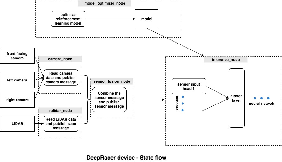
AWS DeepRacer. Allows exploration of RL. Simplifies the mapping of camera input to computer input, so one can focus more on the reward function and deep learning aspects. The car has a set of possible actions (change heading, change speed). The RL task is to predict the actions based on the inputs.
What are some of the strategies applied to winning DeepRacer ?
“DeepRacer: Educational Autonomous Racing Platform for Experimentation with Sim2Real Reinforcement Learning” – https://arxiv.org/pdf/1911.01562.pdf
DeepRacer uses RLLib which brings forth a key idea of encapsulating parallelism in the context of AI applications, as described in RLlib: Abstractions for Distributed Reinforcement Learning. RLLib is part of Ray, described in Ray: A Distributed Framework for Emerging AI Applications . Encapsulating parallelism means that individual components specify their own internal parallelism and resources requirements and can be used by other components without any knowledge of these. This allows a larger system to be built from modular components.
OpenAI Gym offers a suite of environments for developing and comparing RL algorithms. It emphasizes environments over agents, complexity over performance, knowledge sharing over competition. https://github.com/openai/gym , Open AI Gym paper. Here’s a code snippet from this paper of how they see an agent interact with the environments over 100 steps of a training episode.
ob0 = env.reset() # sample environment state, return first observation
a0 = agent.act(ob0) # agent chooses first action
ob1, rew0, done0, info0 = env.step(a0) # environment returns observation,
# reward, and boolean flag indicating if the episode is complete.
a1 = agent.act(ob1)
ob2, rew1, done1, info1 = env.step(a1)
...
a99 = agent.act(o99)
ob100, rew99, done99, info2 = env.step(a99)
# done99 == True => terminal
RL is not a fit for every problem. Alternative approaches with better explainability and determinism include behavior trees, vectorization/VectorNet, …
Deep learning is being applied to combinatorial optimization problems. A very intriguing talk by Anna Goldie discussed an application of RL to chip design that cuts down the time for layout optimization and which in turn enables optimizing of the chip design for a target software stack in simulation before the chip goes to production. Here’s a paper – graph placement methodology for fast chip design.
A snippet on how the research direction evolved to a learning problem.
“Chip floorplanning as a learning problem
The underlying problem is a high-dimensional contextual bandits problem but, as in prior work, we have chosen to reformulate it as a sequential Markov decision process (MDP), because this allows us to more easily incorporate the problem constraints as described below. Our MDP consists of four key elements: (1) States encode information about the partial placement, including the netlist (adjacency matrix), node features (width, height, type), edge features (number of connections), current node (macro) to be placed, and metadata of the netlist graph (routing allocations, total number of wires, macros and standard cell clusters). (2) Actions are all possible locations (grid cells of the chip canvas) onto which the current macro can be placed without violating any hard constraints on density or blockages. (3) State transitions define the probability distribution over next states, given a state and an action. (4) Rewards are 0 for all actions except the last action, where the reward is a negative weighted sum of proxy wirelength, congestion and density, as described below.
We train a policy (an RL agent) modelled by a neural network that, through repeated episodes (sequences of states, actions and rewards), learns to take actions that will maximize cumulative reward (see Fig. 1). We use proximal policy optimization (PPO) to update the parameters of the policy network, given the cumulative reward for each placement.”
Their diagram:
“An embedding layer encodes information about the netlist adjacency, node features and the current macro to be placed. The policy and value networks then output a probability distribution over available grid cells and an estimate of the expected reward for the current placement, respectively. id: identification number; fc: fullyconnected layer; de-conv: deconvolution layer”
“Fig. 1 | Overview of our method and training regimen.In each training iteration, the RL agent places macros one at a time (actions, states and rewards are denoted byai, si and ri, respectively). Once all macros are placed, the standard cells are placed using a force-directed method. The intermediate rewards are zero. The reward at the end of each iteration is calculated as a linear combination of the approximate wirelength, congestion and density, and is provided as feedback to the agent to optimize its parameters for the next iteration.”
PyTorch is an open source machine learning framework that is primarily used for building deep learning models. The framework is built on top of the Torch library and is implemented in Python, with support for C++ and CUDA.
The main C++ classes in PyTorch are:
Tensor: This is the core object in PyTorch and represents a multi-dimensional array. Tensors are the basic building blocks of a PyTorch model and are used to store and manipulate data.
Autograd: This is PyTorch’s automatic differentiation engine, which allows developers to compute gradients of tensors with respect to a loss function. The autograd module also provides a set of functions for computing gradients of complex functions.
nn.Module: This is a base class for all neural network modules in PyTorch. It provides a convenient way to define and organize layers of a neural network, as well as a set of useful methods for training and evaluating the model.
Optimizer: This is a class that implements various optimization algorithms, such as stochastic gradient descent (SGD), Adam, and Adagrad. The optimizer is used to update the parameters of a model during training.
DataLoader: This is a utility class that provides an efficient way to load and preprocess large datasets for training a model. The DataLoader class can be used to batch and shuffle data, as well as to apply various transformations to the data.
PyTorch’s autograd engine implements a variant of reverse-mode automatic differentiation, which is also known as backpropagation. This algorithm efficiently calculates the gradients of the output with respect to each input variable by traversing the computational graph in reverse order, propagating the gradients backwards through each operation using the chain rule.