Tag: ml

Absolute Zero: zero reliance on external data to improve model reasoning

Imagine you want to train a large language model to get really good at solving tough problems—things like math puzzles or writing correct code. Usually, the way people do this is by giving the model lots of practice questions written by humans. These are called human-curated tasks: real people come up with the problems and answers, like “Write a program to reverse a string” or “What’s the derivative of x²?”. The model practices on these problem-solution pairs, and then reinforcement learning (RL) or reinforcement learning with verifiable rewards (RLVR) can be used to improve how it reasons.

But as models get bigger and smarter, collecting enough high-quality problems from humans becomes expensive, slow, and limiting. If the model might one day surpass most humans, why should humans be the bottleneck?

That’s where this paper’s idea, called Absolute Zero, comes in. Instead of relying on people to write problems, the model creates its own. One part of the model plays the “teacher,” proposing new tasks, and another part plays the “student,” trying to solve them. Because the environment is code, the answers can be automatically checked just by running the program—so no human needs to grade them.

The model learns three kinds of reasoning:

  • Deduction: given a program and input, figure out the output.
  • Abduction: given a program and an output, figure out the input.
  • Induction: given some examples, figure out the program that works in general.

The system rewards the student for solving problems correctly, and the teacher for coming up with problems that are just the right difficulty—not too easy, not impossible.

The result is that training only on these self-made coding tasks made the model better at math. On standard benchmarks, it matched or even beat other models that were trained with large sets of human-written problems. Bigger models improved even more, and “coder” models (already good at programming) saw the biggest gains. The model even started showing “scratch-pad” style reasoning on its own, writing little notes or plans before coding—without being told to.

In short, the key insight is this: you don’t necessarily need humans to write all the practice problems anymore. If you have a way to automatically check answers, a model can bootstrap itself, creating and solving its own challenges, and still learn to reason across domains.

The authors do warn that there are challenges—like making sure tasks stay diverse, keeping the system safe, and managing the heavy compute costs—but the big takeaway is that self-play with verifiable rewards could be a new path to building smarter, more independent reasoning systems.

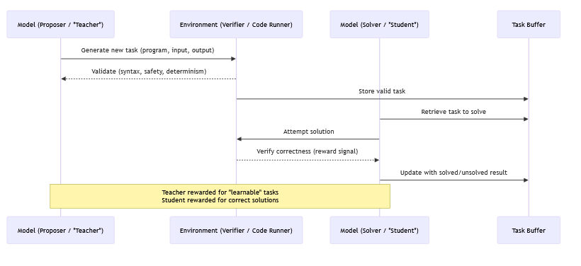
There’s no “exam” in the usual sense for the students – the system builds a feedback loop between the teacher (proposer) and the student (solver).

Here’s how it works step by step:

1. Teacher proposes a task

The proposer (teacher model) generates a new program + input/output pair (a problem).

Example: “Write a function that finds prime numbers up to N.”

2. Environment checks validity

The environment (code runner) ensures the task is valid: it runs, is safe, deterministic, etc.

If valid, it gets stored in a task buffer.

3. Student attempts the task

The solver (student model) pulls the task and tries to solve it.

The environment executes the student’s answer and checks correctness.

4. Rewards reflect difficulty

If the student always solves a task → it’s too easy → proposer gets low reward.

If the student never solves a task → it’s too hard → proposer also gets low reward.

If the student solves it sometimes → it’s “learnable” → proposer gets high reward.

So the proposer doesn’t “know” in advance how good the student is. Instead, it learns over time:

Tasks that end up being useful for training (medium difficulty) get reinforced.

Tasks that are too trivial or impossible fade out because they bring no proposer reward.

The proposer is like a coach who experiments with new drills, and the student’s performance on them acts as the exam. Over time, the teacher learns what kinds of problems best stretch the student without breaking them.

SageMaker Hyperpod for Distributed Model Training

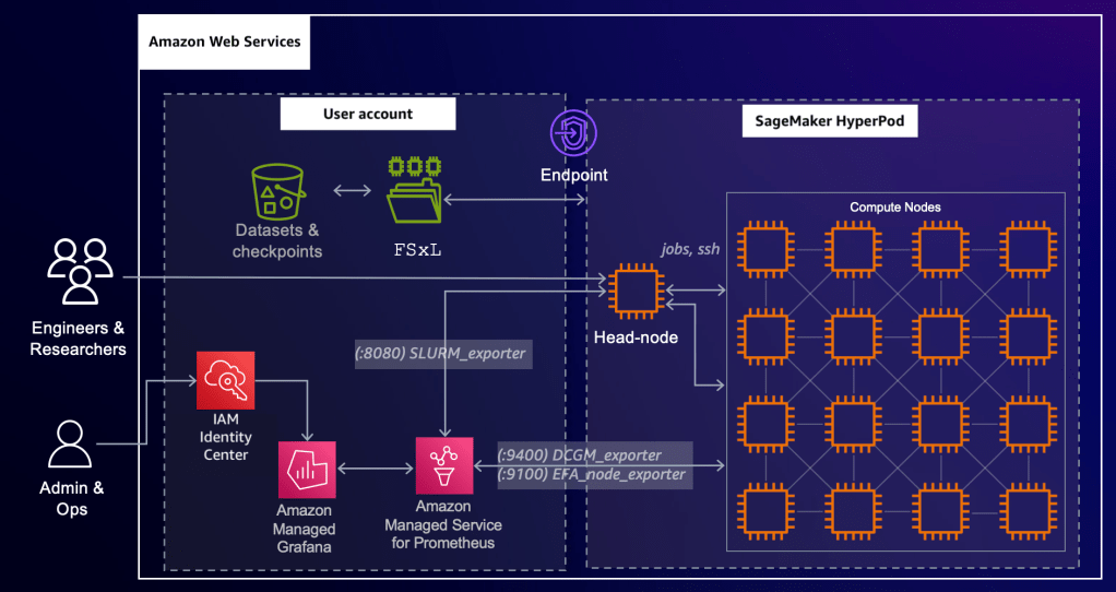
Amazon SageMaker HyperPod is a new infrastructure designed specifically for distributed training at scale. It offers a purpose-built, high-performance environment that accelerates the training of large machine learning models by optimizing resource allocation, reducing communication overhead, and providing seamless scaling. HyperPod integrates with SageMaker to simplify complex training workflows, making it easier for users to efficiently train foundation models and other large-scale ML workloads. This innovation supports faster iteration and development of AI models. https://aws.amazon.com/sagemaker/hyperpod , https://aws.amazon.com/blogs/machine-learning/introducing-amazon-sagemaker-hyperpod-to-train-foundation-models-at-scale

Perplexity, a generative AI startup, improved its model training speed by 40% using Amazon SageMaker HyperPod on AWS. By leveraging advanced distributed training capabilities and EC2 instances, Perplexity optimized its model training and inference processes. This allowed the company to efficiently handle over 100,000 queries per hour with low latency and high throughput, enhancing user experiences and enabling rapid iteration in AI development. https://aws.amazon.com/solutions/case-studies/perplexity-case-study

https://docs.aws.amazon.com/sagemaker/latest/dg/sagemaker-hyperpod-cluster-observability.html

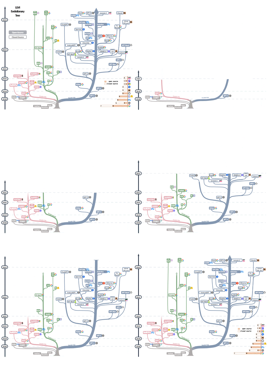
LLM evolution – Anthropic , AI21, Cohere, GPT-4

https://github.com/Mooler0410/LLMsPracticalGuide

Source paper – Harnessing the Power of LLMs in Practice: A Survey on ChatGPT and Beyond

Pink branch is encoder only. Green branch is encoder-decoder. Blue branch is decoder-only.

This is consistent with the Generative aspect of the blue branch. But it does not explain the emergent properties at the top of the blue tree.

LLM leaderboard – https://chat.lmsys.org/?leaderboard

Stanford HELM (holistic evaluation of LMs) – https://crfm.stanford.edu/helm/latest/?models=1

Constitutional AI paper from Anthropic – https://arxiv.org/abs/2212.08073

More on emergent properties in links below.

https://yaofu.notion.site/How-does-GPT-Obtain-its-Ability-Tracing-Emergent-Abilities-of-Language-Models-to-their-Sources-b9a57ac0fcf74f30a1ab9e3e36fa1dc1

https://openai.com/research/solving-math-word-problems : Autoregressive models, which generate each solution token by token, have no mechanism to correct their own errors. Solutions that veer off-course quickly become unrecoverable, as can be seen in the examples provided. We address this problem by training verifiers to evaluate the correctness of model-generated solutions. Verifiers are given many possible solutions, all written by the model itself, and they are trained to decide which ones, if any, are correct.

Language Models are Few-Shot Learners – https://openai.com/research/language-models-are-few-shot-learners

LLM inferencing tools/techniques were discussed here.

LLM Inferencing is hard – tools and techniques

Large Language Models take up a lot of GPU memory with the larger ones exceeding GPU memory sizes. Space is taken up my the model weights as well as by in-memory query specific tensor calculations. Model parallelism to store an LLM across multiple GPUs is both expensive and hard. This makes it important to look at techniques to fit an LLM in a single GPU.

Let’s say the foundation models are available such that no further training is needed and and that one (just) wants to inference against them. Inferencing is not a small challenge, and a number of techniques have been explored. Here’s a link – https://lilianweng.github.io/posts/2023-01-10-inference-optimization/ which discusses

  • student-teacher knowledge distillation training, leading to DistilBert
  • quantization, quantization-aware training, post-training quantization
  • pruning
  • architectural optimization, efficient transformers

OpenAI link on speeding and scaling LLMs to 100k context windows – https://blog.gopenai.com/how-to-speed-up-llms-and-use-100k-context-window-all-tricks-in-one-place-ffd40577b4c

High-throughput Generative Inference of Large Language Models with a Single GPU https://arxiv.org/pdf/2303.06865.pdf, discusses 3 strategies with a focus on a single GPU.

  • model compression
  • collaborative inference
  • offloading to utilize memory from CPU and disk

They then show 3 contributions

  • definition of the optimization search space for offloading, including weights, activations, KV cache, and an algorithm to get an optimal offloading strategy within the search space
  • quantization of the parameters to 4 bits with small loss of accuracy
  • run a OPT-175B model on a single T4 GPU with 16GB memory (!)

PEFT – Scaling Down to Scale Up: A Guide to Parameter-Efficient Fine-Tuning – https://arxiv.org/pdf/2303.15647.pdf says ”expanding the context size leads to a quadratic increase in inference costs

There are three main classes of PEFT methods:

  • Addition-based, ( Within additive methods, we distinguish two large included groups: Adapter-like methods and Soft prompts)
  • Selection-based, and
  • Reparametrization-based.

General strategies for inference concurrency, courtesy chatgpt:

To process multiple concurrent inference requests without interference between them, a model can use techniques such as parallelization and batching.

Parallelization involves splitting the workload across multiple processing units, such as CPUs or GPUs, so that multiple requests can be processed simultaneously without interfering with each other. This can be achieved using frameworks such as TensorFlow or PyTorch, which provide support for parallel processing.

Batching involves grouping multiple requests together and processing them as a single batch. This can increase the efficiency of the model by reducing the overhead associated with processing each request individually. Batching can be particularly effective for models that are optimized for throughput rather than latency.

Another technique that can be used is dynamic scheduling, which involves assigning resources to requests based on their priority and the availability of resources at a given time. This can help ensure that high-priority requests are processed quickly without interfering with lower-priority requests.

Efficiently scaling transformer inference – link is a paper from Google discussing partitioning of weights and activations across multiple heads and multiple chips (Nov’22).

Feature Vectors, Embeddings, Vector Databases, Feature Stores

An ML model consists of a set of weights (or a set of numerical values) that transform inputs to outputs (along with a nonlinear transform such as a sigmoid function). The weights are often organized as vectors or matrices. Consider neural networks, decision trees and support vector machines as types of ML models for this discussion.

The weights representing features of the data (input or intermediate data) are also called feature vectors or vectors. They are also called embeddings, that is embeddings of vectors in a vector space. We discussed such vectors in https://securemachinery.com/2019/05/24/transformer-gpt-2/.

The term “embedding” comes from the idea that the vectors “embed” the original data into a lower-dimensional space. The embedding process involves a combination of statistical and computational techniques, such as factorization and neural networks, that learn to map the input data into the vector space in a way that preserves the relevant properties of the original data.

The use of vectors to represent words in machine learning research started in 2013 with the publication of the paper “Distributed Representations of Words and Phrases and their Compositionality” by Tomas Mikolov et al. This paper introduced the word2vec algorithm, which generates dense vector representations of words based on their distributional properties in a large corpus of text. The size of the vector or embedding in a word embedding model is a hyperparameter that needs to be determined before training the model. It is typically chosen based on the size of the vocabulary and the complexity of the task at hand. In practice, the vector size is often set to be between 100 and 300 dimensions, but this can vary depending on the specific application and the available computational resources. The optimal vector size can be determined through experimentation and tuning of hyperparameters.

One difference between embeddings and feature vectors is that embeddings are typically learned automatically from the data, while feature vectors are typically chosen based on domain knowledge or feature engineering. However these two terms are often used interchangeably. Here is a video going over how the embeddings are obtained from words in a sentence with a bag of words approach- https://www.youtube.com/watch?v=viZrOnJclY0 .

Pinecone, Milvus, Facebook AI Similarity Search (FAISS), Google Vertex Matching engine are examples of Vector databases.

The challenge in implementing a vector database is that traditional databases are not optimized for handling high-dimensional vector data, which is often used in machine learning and data science applications.

Vector data is typically represented as arrays of numbers, where each number represents a feature or attribute of the data. For example, an image might be represented as a high-dimensional vector where each dimension represents the color value of a specific pixel. In contrast to traditional databases, where each record consists of a set of fields or columns, vector databases need to store and index large volumes of high-dimensional data in a way that supports efficient similarity search.

In traditional databases, queries are typically based on simple comparisons of scalar values, such as equality or range queries. However, in vector databases, similarity search is the primary operation, which requires specialized algorithms and data structures to efficiently compute the similarity between vectors. These algorithms are designed to handle high-dimensional data and minimize the amount of computation needed to compare vectors, which can be computationally expensive.

There are several specialized algorithms that are commonly used in vector databases to support efficient similarity search. Here are some examples:

  1. Euclidean Distance: This is a distance metric that measures the straight-line distance between two points in Euclidean space. It is commonly used in vector databases to compute the distance or similarity between vectors.
  2. Cosine Similarity: This is a similarity metric that measures the cosine of the angle between two vectors. It is commonly used in text-based applications to measure the similarity between documents or word embeddings.
  3. Locality-Sensitive Hashing (LSH): This is a technique used to hash high-dimensional vectors into lower-dimensional buckets based on their similarity. It is commonly used in vector databases to speed up similarity search by reducing the number of comparisons needed to find similar vectors.
  4. Product Quantization: This is a technique used to divide high-dimensional vectors into smaller subvectors and quantize them separately. It is commonly used in vector databases to reduce the dimensionality of the data and speed up similarity search.
  5. Inverted Indexing: This is a technique used to index the vectors based on the values of their individual dimensions. It is commonly used in text-based applications to speed up search queries by indexing the terms in the document.

Pinecone provides several indexing and search algorithms, including approximate nearest neighbor search, that are selected automatically based on the properties of the data and the search requirements. However, you can also specify a specific algorithm or tuning parameters when creating an index or performing a query by passing in the appropriate arguments. For example, you can use the method parameter when creating an index to specify the indexing method, or the distance parameter when performing a query to specify the distance metric to use.

While OpenSearch is not specifically designed as a vector database like Pinecone, it provides vector search capabilities through its support for nearest neighbor search. OpenSearch uses the K-Nearest Neighbor (K-NN) algorithm to perform nearest neighbor search for vector data. K-NN is a machine learning algorithm that can be used to find the K nearest neighbors of a query vector in a high-dimensional space. OpenSearch also provides support for approximate nearest neighbor search using algorithms such as Annoy and Hnswlib. To use vector search in OpenSearch, you first need to index your vector data using the appropriate data type (e.g., float or double). You can then perform a nearest neighbor search by specifying the query vector and the number of nearest neighbors to return. OpenSearch also provides support for vector scoring, which allows you to rank search results based on their similarity to a query vector. You can use vector scoring to boost or filter search results based on their similarity to a query vector.

What kind of vectorization schemes are useful for log processing ?

When processing log data, the goal is typically to extract useful information from the log entries and transform them into a format that can be easily analyzed and searched. Vectorization is a common technique used for this purpose, and there are several vectorization schemes that are applicable to log processing. Here are some examples:

  1. Bag-of-words: This is a vectorization scheme that represents a document as a bag of words, where each word is represented by a dimension in the vector and the value of the dimension is the frequency of the word in the document. Bag-of-words can be used to represent log entries as a vector of words, which can be used for tasks such as text classification and anomaly detection.
  2. TF-IDF: This is a vectorization scheme that represents a document as a weighted combination of its term frequency and inverse document frequency. TF-IDF can be used to represent log entries as a vector of weighted words, which can be used for tasks such as information retrieval and text mining.
  3. Word embeddings: This is a vectorization scheme that represents words as dense vectors in a high-dimensional space, where the distance between vectors reflects the semantic similarity between the words. Word embeddings can be used to represent log entries as a vector of word embeddings, which can be used for tasks such as text classification and entity recognition.
  4. Sequence embeddings: This is a vectorization scheme that represents a sequence of words as a dense vector in a high-dimensional space, where the distance between vectors reflects the similarity between the sequences. Sequence embeddings can be used to represent log entries as a vector of sequence embeddings, which can be used for tasks such as sequence classification and anomaly detection.
  5. One-hot encoding: This is a vectorization scheme that represents categorical data as binary vectors, where each dimension corresponds to a possible category and the value of the dimension is 1 if the data belongs to that category and 0 otherwise. One-hot encoding can be used to represent log entries as a vector of categorical features, which can be used for tasks such as classification and clustering.

By using a suitable vectorization scheme, log data can be transformed into a format that can be easily analyzed and searched, enabling tasks such as anomaly detection, root cause analysis, and performance optimization.

Vector database versus Feature store – what’s the difference ?

Both vector databases and feature stores are used to manage and serve high-dimensional data, such as embeddings, vectors, and other numerical representations, but there are some key differences between the two.

A vector database is a database optimized for storing and querying high-dimensional vector data. It provides efficient indexing and search algorithms, such as approximate nearest neighbor search, that allow for fast and scalable similarity search. Vector databases are commonly used in machine learning applications, such as recommendation systems and natural language processing, where the goal is to find similar items or entities based on their vector representations.

A feature store, on the other hand, is a centralized repository for machine learning features that provides a way to store, manage, and share feature data across different applications and teams. It is designed to help data scientists and machine learning engineers build, test, and deploy machine learning models more efficiently by providing a unified interface for accessing and managing features.

While both vector databases and feature stores can store and serve high-dimensional data, the main difference is their focus and use case. Vector databases are designed for efficient similarity search, while feature stores are designed for feature management and sharing across different applications and teams. In practice, they can complement each other in many machine learning workflows, with the vector database providing the efficient similarity search capabilities and the feature store providing a centralized and standardized way to manage and share feature data.

Comparison of Milvus Pinecone Vespa Weaviate Vald GSI Qdrant – https://towardsdatascience.com/milvus-pinecone-vespa-weaviate-vald-gsi-what-unites-these-buzz-words-and-what-makes-each-9c65a3bd0696

Anyscale – Using an embeddings database to train an LLM using Ray – https://www.anyscale.com/blog/llm-open-source-search-engine-langchain-ray

OpenAI embeddings example – https://github.com/openai/openai-cookbook/blob/main/examples/Question_answering_using_embeddings.ipynb

HuggingFace sentence embeddings article – https://medium.com/huggingface/universal-word-sentence-embeddings-ce48ddc8fc3a

AWS – https://medium.com/@shankar.arunp/augmenting-large-language-models-with-verified-information-sources-leveraging-aws-sagemaker-and-f6be17fb10a8
EC2 P5 UltraClusters

Each P5 EC2 instances has

  • eight NVIDIA H100 GPUs capable of 16 petaFLOPs of mixed-precision performance
  • 640 GB of high-bandwidth memory, 80GB in each GPU
  • 3,200 Gbps networking connectivity (8x more than the previous generation)

The increased performance of P5 instances accelerates the time-to-train machine learning (ML) models by up to 6x (reducing training time from days to hours), and the additional GPU memory helps customers train larger, more complex models.

P5 instances are expected to lower the cost to train ML models by up to 40% over the previous generation, providing customers greater efficiency over less flexible cloud offerings or expensive on-premises systems.

https://nvidianews.nvidia.com/news/aws-and-nvidia-collaborate-on-next-generation-infrastructure-for-training-large-machine-learning-models-and-building-generative-ai-applications

Nvidia H100 GPU overview and data sheet – https://resources.nvidia.com/en-us-tensor-core/gtc22-whitepaper-hopper

Diagram of P4d UltraClusters

P4d consists of 8 A100 GPUs, with 40GB GPU Memory each

P4de consists of 8 A100 80GB GPUs, with 80GB GPU memory each

Nvidia blog on HGX baseboard supporting 8 A100 GPUs – https://developer.nvidia.com/blog/introducing-hgx-a100-most-powerful-accelerated-server-platform-for-ai-hpc/

A100 80GB data sheet – https://www.nvidia.com/en-us/data-center/a100/

MIG support in A100 – https://developer.nvidia.com/blog/getting-the-most-out-of-the-a100-gpu-with-multi-instance-gpu/ and MIG user guide – https://docs.nvidia.com/datacenter/tesla/mig-user-guide

MIG support in AWS EC2 instance type P4d and in AWS EKS – https://developer.nvidia.com/blog/amazon-elastic-kubernetes-services-now-offers-native-support-for-nvidia-a100-multi-instance-gpus/

GCP A2 adds 16 A100 GPUs to a node – https://cloud.google.com/blog/products/compute/announcing-google-cloud-a2-vm-family-based-on-nvidia-a100-gpu

https://cloud.google.com/blog/products/containers-kubernetes/gke-now-supports-multi-instance-gpus

Running more pods/gpu on EKS with MIG – https://medium.com/itnext/run-more-pods-per-gpu-with-nvidia-multi-instance-gpu-d4f7fb07c9b5

Nvidia Embraces The CPU World With “Grace” Arm Server Chip

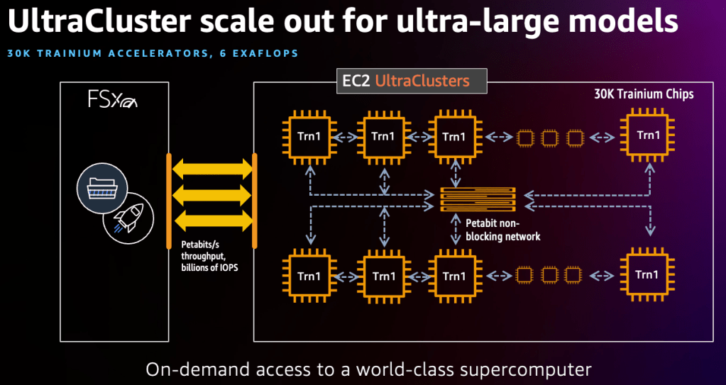
EC2 Trainium UltraClusters

Each EC2 Trn1 instance has

  • up to 16 AWS Trainium accelerators purpose built to accelerate DL training and deliver up to 3.4 petaflops of FP16/BF16 compute power. Each accelerator includes two second-generation NeuronCores
  • 512 GB of shared accelerator memory (HBM) with 9.8 TB/s of total memory bandwidth
  • 1600 Gbps of Elastic Fabric Adapter (EFAv2)

An EC2 Trn1 UltraCluster, consists of densely packed, co-located racks of Trn1 compute instances interconnected by non-blocking petabyte scale networking. It is our largest UltraCluster to date, offering 6 exaflops of compute power on demand with up to 30,000 Trainium chips.

https://aws.amazon.com/blogs/machine-learning/scaling-large-language-model-llm-training-with-amazon-ec2-trn1-ultraclusters/

Weights vs Activations

Why do Activations need more bits (16) than weights (8) ? source – https://stackoverflow.com/questions/72397839/why-do-activations-need-more-bits-16bit-than-weights-8bit-in-tensor-flows-n

Answer:

Activations are actual signals propagating through the network. They have nothing to do with activation function, this is just a name collision. They are higher accuracy because they are not part of the model, so they do not affect storage, download size, or memory usage, as if you are not training your model you never store activations beyond the current one.

For example for an MLP (middle layer perceptron ?) we have something among the lines of

a1 = relu(W1x + b1)
a2 = relu(W2a1 + b2)
...
an = Wnan-1 + bn

where each W and b will be 8bit parameters. And activations are a1, …, an. The thing is you only need previous and current layer, so to calculate at you just need at-1, and not previous ones, consequently storing them during computation at higher accuracy is just a good tradeoff.

Datastore for Activations:

  • During training, activations are typically stored in the GPU’s memory for models trained on GPUs. This is because backpropagation requires these activations for gradient computation. Given that modern deep learning models can have millions to billions of parameters, storing all these activations can be memory-intensive.
  • During inference, you only need to perform a forward pass and don’t need to store all activations, except for the ones necessary for computing subsequent layers. Once an activation has been used to compute the next layer, it can be discarded if not needed anymore.

Hugging Face – AI models and datasets hub

Hugging Face supports around 100,000 pre-trained language models that can be used for various NLP tasks. The Hugging Face transformers library, which is a popular choice for NLP tasks such as text classification and machine translation, currently supports over 100 pre-trained language models. These models include popular models such as BERT, GPT-2, and RoBERTa. In addition Hugging Face provides tools and libraries that allow users to fine-tune and customize these models for specific tasks or datasets.

The datasets can be loaded using the python datasets package (pip install datasets). An overview is here.

A Hugging Face Course – https://github.com/huggingface/course

Hugging Face on AWS blog – https://aws.amazon.com/blogs/machine-learning/aws-and-hugging-face-collaborate-to-simplify-and-accelerate-adoption-of-natural-language-processing-models/

CEO Clement Delangue, calls it the “GitHub of machine learning.” Its emphasis on an open, collaborative approach that made investors confident in the company’s $2 billion valuation, he said. “That’s what is really important to us, makes us successful and makes us different from others in the space.” 

DistilBERT is a smaller, faster, and cheaper version of the BERT language model developed by Hugging Face by controlling the loss function during training of a ‘student model’ from a ‘teacher model’. It bucks the trend towards larger models, and instead focusses on training a more efficient model. It has been “distilled” to reduce its size and computational requirements, making it faster to train and more efficient to run. Despite being smaller than BERT, DistilBERT is able to achieve similar or even slightly better performance on many NLP tasks. The triple loss function is devised to include a distillation loss, a training loss and a cosine-distance loss.

Examples of generative models available on the Hugging Face platform include:

  1. GPT-2: GPT-2 (Generative Pre-training Transformer 2) is a large-scale language model developed by OpenAI that can be used for tasks such as language translation and text generation.
  2. BERT: BERT (Bidirectional Encoder Representations from Transformers) is a language model developed by Google that can be used for tasks such as language translation and text classification.
  3. RoBERTa: RoBERTa (Robustly Optimized BERT Approach) is a language model developed by Facebook that is based on the BERT model and can be used for tasks such as language translation and text classification.
  4. T5: T5 (Text-To-Text Transfer Transformer) is a language model developed by Google that can be used for tasks such as language translation and text summarization.
  5. DistilBERT, described above. To generate text with DistilBERT, you would typically fine-tune the model on a specific task, such as machine translation or language generation, using a dataset that is relevant to the task. Once the model has been fine-tuned, you can use it to generate text by providing it with a prompt or seed text and letting it predict the next word or sequence of words.

Docs on text generation – https://huggingface.co/transformers/v3.1.0/main_classes/model.html?highlight=generate

Here’s an example of using transformers to generate some text.

import transformers

# Load the model and tokenizer
tokenizer = AutoTokenizer.from_pretrained('distilgpt2') 
model = AutoModelWithLMHead.from_pretrained('distilgpt2')  

# Encode the prompt
input_context_prompt = "Men on the moon "
input_ids = tokenizer.encode(input_context_prompt, return_tensors='pt')  # encode input context

# Generate text
outputs = model.generate(input_ids=input_ids, max_length=40, temperature=0.9, num_return_sequences=10, do_sample=True)  

# Sample candidate outputs and print
for i in range(10): #  10 output sequences were generated
    print('Generated {}: {}'.format(i, tokenizer.decode(outputs[i], skip_special_tokens=True)))

Note the temperature parameter during model.generate(). A temperature of zero means the generation process will choose the most likely next word . A higher temperature allows for less likely words to be included in the generation process.

Machine Learning Security

Seven security concerns in Machine Learning (ML) –

  1. Data privacy and security: ML requires large amounts of data to be trained, and this data may contain sensitive or personal information. Appropriate measures need to be put in place to prevent data from being accessed by unauthorized parties.
  2. Notebooks security: ML typically requires Jupyter or similar notebooks to be served for data scientists to work on data, code, and models, both individually and collaboratively. These notebooks need to be access controlled and protected from unauthorized access. This includes the code and git repos that host the code, and the model artifacts that the notebook uses or creates.
  3. Model serving and inference security: ML models in production are commonly served and accessed over inference endpoints and such endpoints need authentication, authorization, encryption for protection against misuse. During model upgrades to an endpoint or changes to an endpoint and its configuration, a number of attacks are possible that are typical of a devops/devsecops pipeline. These need to be protected against.
  4. Model security: Models can be vulnerable to attacks such as adversarial inputs, such as when an attacker intentionally manipulates the input to the model in order to cause it to make incorrect predictions. Another example is when the model makes an egregiously bad decision on an input, for example a self-driving car hitting an obstacle instead of avoiding it. It is important to harden the model and bound the decisions that come from its use.
  5. Misuse: Even if a model works as designed, it can be misused, for example by generating fake or misleading content. It is important to consider the potential unintended consequences of using models and to put safeguards in place to prevent their misuse.
  6. Bias: ML models can sometimes exhibit biases due to the data they are trained on. There should be a plan to identify biases in a model and take steps to mitigate them.
  7. Intellectual property: ML models may be protected by intellectual property laws, and it is important to respect these laws and obtain the appropriate licenses when using language models developed by others.

Distributed Training – Parameter server, Data and Model parallelism

Distributed Training aims to reduce the time to train an model in machine learning, by splitting the training workload across multiple nodes. It has gained in importance as data sizes, model sizes and complexity of training have grown. Training consists of iteratively minimizing an objective function by running the data through a model and determining a) the error and the gradients with which to adjust the model parameters (forward path) and b) the updated model parameters using calculated gradients (reverse path). The reverse path always requires synchronization between the nodes, and in some cases the forward path also requires such communication.

There are three approaches to distributed training – data parallelism, model parallelism and data-model parallelism. Data parallelism is the more common approach and is preferred if the model fits in GPU memory (which is increasingly hard for large models).

In data parallelism, we partition the data on to different GPUs and and run the same model on these data partitions. The same model is present in all GPU nodes and no communication between nodes is needed on the forward path. The calculated parameters are sent to a parameter server, which averages them, and updated parameters are retrieved back by all the nodes to update their models to the same incrementally updated model.

In model parallelism, we partition the model itself into parts and run these on different GPUs. This applies to large models such as large language models (LLMs) that do not fit in a single GPU.

A paper on Parameter Servers is here, on Scaling Distributed Machine Learning with the Parameter Server.

To communicate the intermediate results between nodes the MPI primitives are leveraged, including AllReduce.

The amount of training data for BERT is ~600GB. BERT-Tiny model is 17MB, BERT-Base model is ~400MB. During training a 16GB memory GPU sees an OOM error.

Some links to resources –

https://andrew.gibiansky.com/blog/machine-learning/baidu-allreduce/

https://github.com/horovod/horovod/blob/master/docs/concepts.rst (Horovod, an open source parameter server).

https://medium.com/pytorch/how-lyft-uses-pytorch-to-power-machine-learning-for-their-self-driving-cars-80642bc2d0ae

https://docs.aws.amazon.com/sagemaker/latest/dg/distributed-training.html

https://aws.amazon.com/blogs/machine-learning/launching-tensorflow-distributed-training-easily-with-horovod-or-parameter-servers-in-amazon-sagemaker/

https://openai.com/blog/scaling-kubernetes-to-2500-nodes/

https://towardsdatascience.com/distributed-deep-learning-training-with-horovod-on-kubernetes-6b28ac1d6b5d

https://mccormickml.com/2019/11/05/GLUE/ Origin of General Language Understanding Evaluation.

https://github.com/google-research/bert

https://towardsdatascience.com/model-parallelism-in-one-line-of-code-352b7de5645a

https://developer.nvidia.com/blog/scaling-language-model-training-to-a-trillion-parameters-using-megatron/

Horovod core principles are based on the MPI concepts size, rank, local rank, allreduce, allgather, and broadcast. These are best explained by example. Say we launched a training script on 4 servers, each having 4 GPUs. If we launched one copy of the script per GPU:

  • Size would be the number of processes, in this case, 16.
  • Rank would be the unique process ID from 0 to 15 (size – 1).
  • Local rank would be the unique process ID within the server from 0 to 3.
  • Allreduce is an operation that aggregates data among multiple processes and distributes results back to them. Allreduce is used to average dense tensors. Here’s an illustration from the MPI Tutorial:
Allreduce Illustration
  • Allgather is an operation that gathers data from all processes in a group then sends data back to every process. Allgather is used to collect values of sparse tensors. Here’s an illustration from the MPI Tutorial:
Allgather Illustration
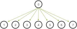
  • Broadcast is an operation that broadcasts data from one process, identified by root rank, onto every other process. Here’s an illustration from the MPI Tutorial:

Horovod switched from using MPI to using NCCL (NVidia Collective Communications Library) for distributing initial weights and biases, and intermediate weights and biases after each training step .

NCCL is a library that provides primitives for communication between multiple GPUs both within a node and across different nodes.

Horovod continues to use MPI for other functions that do not involve inter-GPU communication, such as informing processes on different nodes of their id (aka rank), master vs non-master status for coordination between processes and for sharing the total number of nodes.

NVidia NCCL uses NVLink which is the hardware interconnect that connects multiple GPUs.

NVLink is a high-speed, point-to-point interconnect technology developed by NVIDIA that is designed to enable high-bandwidth communication between processors, GPUs, and other components in a system.

NVLink 1.0, which was introduced in 2016, provides a maximum bidirectional bandwidth of 80 GB/s per link. This means that data can be transferred between two devices at a rate of up to 80 GB/s in each direction.

NVLink 2.0, which was introduced in 2017, provides a maximum bidirectional bandwidth of 300 GB/s per link. This represents a significant increase in bandwidth compared to NVLink 1.0, and allows for even faster data transfer rates between devices.

NVLink 3.0, which was introduced in 2021, provides a maximum bidirectional bandwidth of 600 GB/s per link, making it the fastest version of NVLink to date.

Processors for Deep Learning: Nvidia Ampere GPU, Tesla Dojo, AWS Inferentia, Cerebras

The NVidia Volta-100 GPU released in Dec 2017 was the first microprocessor with dedicated cores purely for matrix computations called Tensor Cores. The Ampere-100 GPU released May’20 is its successor. Ampere has 84 Streaming Multiprocessors (SMs) with 4 Tensor Cores (TCs) each for a total of 336 TCs. Tensor Cores reduce the cycle time for matrix multiplications, operating on 4×4 matrices of 16bit floating point numbers. These GPUs are aimed at Deep Learning use cases which consist of a pipeline of matrix operations.

Here’s an article on choosing the right EC2 instance type for DL – https://towardsdatascience.com/choosing-the-right-gpu-for-deep-learning-on-aws-d69c157d8c86 (G4 for inferencing, P4 for training).

How did the need for specialized DL chips arise, and why are Tensors important in DL ? In math, we have Scalars and Vectors. Scalars are used for magnitude and Vectors encode magnitude and direction. To transform Vectors, one applies Linear Transformations in the form of Matrices. Matrices for Linear Transformations have EigenVectors and EigenValues which describe the invariants of the transformation. A Tensor in math and physics is a concept that exhibits certain types invariance during transformations. In 3 dimensions, a Stress Tensor has 9 components, which can be representated as a 3×3 matrix; under a change of basis the components of the tensor change however the tensor itself does not.

In Deep Learning applications a Tensor is basically a Matrix. The Generalized Matrix Multiplication (GEMM) operation, D=AxB+C, is at the heart of Deep Learning, and Tensor Cores are designed to speed these up.

In Deep Learning, multilinear maps are interleaved with non-linear transforms to model arbitrary transforms of input to output and a specific model is arrived by a process of error reduction on training of actual data. This PyTorch Deep Learning page is an excellent resource to transition from traditional linear algebra to deep learning software – https://pytorch.org/tutorials/beginner/nlp/deep_learning_tutorial.html .

Tesla Dojo is planned to build a processor/computer dedicated for Deep Learning to train on vast amounts of video data. Launched on Tesla AI Day, Aug’20 2021, a video at https://www.youtube.com/watch?v=DSw3IwsgNnc

AWS Inferentia is a chip for deep learning inferencing, with its four Neuron Cores.

AWS Trainium is an ML chip for training.

Generally speaking the desire in deep learning community is to have simpler processing units in larger numbers.

Updates: Cerebras announced a chip which can handle neural networks with 120 trillion parameters, with 850,000 AI optimized cores per chip.

SambaNova, Anton, Cerebras and Graphcore presentations are at https://www.anandtech.com/show/16908/hot-chips-2021-live-blog-machine-learning-graphcore-cerebras-sambanova-anton

SambaNova is building 400,000 AI cores per chip.

NVIDIA GPUAWS InstanceAzure Instance
M60G3
T4G4NVv4
V100P3NCv4
A100P4, P4dNDv4

https://lambdalabs.com/blog/nvidia-a100-vs-v100-benchmarks

Accuracy vs Recall vs Precision vs F1 in Machine Learning

We want to walk through some common metrics in classification problems – such as accuracy, precision and recall – to get a feel for when to use which metric. Say we are looking for a needle in a haystack. There are very few needles in a large haystack full of straws. An automated machine is sifting through the objects in the haystack and predicting for each object whether it is a straw or a needle. A reasonable predictor will predict a small number of objects as needles and a large number as straws. A prediction has two attributes – positive/negative and accurate/inaccurate.

Positive Prediction: the object at hand is predicted to be the needle. A small number.

Negative Prediction: the object at hand is predicted not to be a needle. A large number.

True_Positive: of the total number of predictions, the number of predictions that were positive and correct. Correctly predicted Positives (needles). A small number.

True_Negative: of the total number of predictions, the number of predictions that were negative and correct. Correctly predicted Negatives (straws). A large number.

False_Positive: of the total number of predictions, the number of predictions that are positive but the prediction is incorrect. Incorrectly predicted Positives (straw predicted as needle). Could be large as the number of straws is large, but assuming the total number of predicted needles is small, this is less than or equal to predicted needles, hence small.

False_Negative: of the total number of predictions, the number of predictions that are negative but the prediction is incorrect. Incorrectly predicted Negatives (needle predicted as straw). Is this a large number ? It is unknown – this class is not large just because the class of negatives is large – it depends on the predictor and a “reasonable” predictor which predicts most objects as straws, could also predict many needles as straws. This is less than or equal to the total number of needles, hence small.

Predicted_Positives = True_Positives + False_Positives = Total number of objects predicted as needles.

Actual Positives = Actual number of needles, which is independant of the number of predictions either way, however Actual Positives = True Positives + False Negatives.

Accuracy = nCorrect _Predictons/nTotal_Predictions=(nTrue_Positives+nTrue_Negatives) / (nPredicted_Positives +nPredicted_Negatives) .   # the reasonable assumption above is equivalent to a high accuracy. Most predictions will be hay, and be correct in this simply because of the skewed distribution. This does not shed light on FP or FN.

Precision = nTrue_Positives / nPredicted_Positives    # correctly_identified_needles/predicted_needles;  this sheds light on FP; Precision = 1 => FP=0 => all predictions of needles are in fact needles; a precision less than 1 means we got a bunch of hay with the needles – gives hope that with further sifting the hay can be removed.  Precision is also called Specificity and quantifies the absence of False Positives or incorrect diagnoses.

Recall = nTrue_Positives / nActual_Positives  = TP/(TP+FN)# correctly_identified_needles/all_needles; this sheds light on FN; Recall = 1 => FN = 0; a recall less than 1 is awful as some needles are left out in the sifting process. Recall is also called Sensitivity .

Precision > Recall => FN is higher than FP

Precision < Recall => FN is lower than FP

If at least one needle is correctly identified as a needle, both precision and recall will be positive; if zero needles are correctly identified, both precision and recall are zero.

F1 Score is the harmonic mean of Precision and Recall.  1/F1 = 1/2(1/P + 1/R) . F1=2PR/(P+R) .  F1=0 if P=0 or R=0. F1=1 if P=1 and R=1.

ROC/AUC rely on Recall (=TP/TP+FN) and another metric False Positive Rate defined as FP/(FP+TN)  = hay_falsely_identified_as_needles/total_hay . As TN >> FP, this should be close to zero and does not appear to be a useful metric in the context of needles in a haystack; as are ROC/AuC . The denominators are different in Recall and FPR, total needles and total hay respectively.

There’s a bit of semantic confusion when saying True Positive or False Positive. These shorthands can be interpreted as- it was known that an instance was a Positive and a label of True or False was applied to that instance. But what we mean is that it was not known whether the instance was a Positive, and that a determination was made that it was a Positive and this determination was later found to be correct (True) or incorrect (False). Mentally replace True/False with ‘Correct/Incorrectly identified as’ to remove this confusion.

Normalization: scale of 0-1, or unit norm; useful for dot products when calculating similarity.

Standardization: zero mean, divided by standard deviation; useful in neural network/classifier inputs

Regularization: used to reduce sensitivity to certain features. Uses regression. L1: Lasso regression L2: Ridge regression

Confusion matrix: holds number of predicted values vs known truth. Square matrix with size n equal to number of categories.

Bias, Variance and their tradeoff. we want both to be low. When going from a simple model to a complex one, one often goes from high bias to a high variance scenario. https://towardsdatascience.com/understanding-the-bias-variance-tradeoff-165e6942b229

ML Transformer and GPT-2 Meetup

AI meetup, GPT-2 demo and discussion. Attention!

“The attention mechanism allows the model to create the context vector as a weighted sum of the hidden states of the encoder RNN at each previous timestamp.”

“Transformer is a type of model based entirely on attention, and does not require recurrent or convolutional layers”

Context vector is the output of the Encoder in an Encoder-Decoder network (EDN). EDNs struggle to retain all the required information for the decoder to accurately decode. Attention is a mechanism to solve this problem.

“Attention mechanisms let a model directly look at, and draw from, the state at any earlier point in the sentence. The attention layer can access all previous states and weighs them according to some learned measure of relevancy to the current token, providing sharper information about far-away relevant tokens.”

GPT: Generative Pre-Trained Transformer. Unlike BERT, it is generative and not geared to comprehension, translation or summarization tasks, but instead writing or generative tasks. It uses unsupervised learning to train a deep neural network with a seq2seq model. It does not use reinforcement learning (feedback from environment) or supervised learning. It uses “masked self-attention” to predict the next text during training on its dataset.

The term “generative” is used to emphasize GPT’s ability to generate new, original text, rather than just processing or analyzing text that already exists. A generative model is a type of machine learning model that is trained to produce data, such as text, images, or music, that is similar to the data it was trained on. GPT is a generative model because it is trained on a large corpus of text data and can then generate new text that is similar to the text in its training data. This allows GPT to produce human-like text on a wide range of topics, which can be useful for a variety of applications, such as language translation, text summarization, and question answering.

A “transformer” is a type of neural network architecture that was introduced in 2017. It is a deep learning model that is used for natural language processing tasks, such as language translation and text summarization. A transformer consists of two main components: an encoder, which processes the input text, and a decoder, which generates the output text. The encoder and decoder are connected by a series of attention mechanisms, which allow the model to focus on different parts of the input text as it generates the output. This architecture allows the model to process input text in a parallel, rather than sequential, manner, which makes it more efficient and effective than previous models. The transformer architecture has been widely adopted in natural language processing and has been shown to be highly effective for many tasks.

In a transformer, the “attention” mechanism allows the model to focus on different parts of the input text at different times as it generates the output text. This is different from previous neural network models, which processed the input text sequentially, one word at a time. The attention mechanism in a transformer works by calculating a weight for each word in the input text. This weight represents the importance of that word in the context of the current output word that the model is generating. The model then uses these weights to decide which words in the input text to focus on as it generates the output. This allows the model to selectively focus on the most relevant words in the input text.

https://en.m.wikipedia.org/wiki/Transformer_(machine_learning_model) was initially released June 2017 by Google Brain team.

GPT was released June 2018 by OpenAI.

BERT was released Oct 2018 by Google.

GPT-2 was announced Feb 2019 by OpenAI, trained on 40GB of text.

GPT-3 was introduced May 2020 and in beta testing in July 2020. Trained on 10x the data, or 400GB.

BERT is a response to GPT and GPT-2 is in turn a response to BERT.

This attention concept looks akin to a fourier or laplace transform which encodes the entire input signal in a lossless manner in a way that allows sections or bands of it to be referred to later. Although implemented differently it’s a way to keep track of and refer to global state.

AutoML and Transformer – http://ai.googleblog.com/2019/06/applying-automl-to-transformer.html

Transformer architecture

BERT and GPT are both based on the Transformer ideas. BERT is bidirectional and better at ccomprehending meaning from the whole sentence/phrase whereas GPT is better at generating text.

https://jalammar.github.io/illustrated-transformer/

https://jalammar.github.io/visualizing-neural-machine-translation-mechanics-of-seq2seq-models-with-attention/

Bahdanau, 2014 introduced the concept of Attention https://arxiv.org/abs/1409.0473

“The most important distinguishing feature of this approach from the basic encoder–decoder is that it does not attempt to encode a whole input sentence into a single fixed-length vector. Instead, it encodes the input sentence into a sequence of vectors and chooses a subset of these vectors adaptively while decoding the translation. This frees a neural translation model from having to squash all the information of a source sentence, regardless of its length, into a fixed-length vector. We show this allows a model to cope better with long sentences.”

This description makes it more like a wavelet transform, that does auto-correleations of a signal at different levels of granularity to make sense of it.

Conceptual progression

  1. Input -> Encoder -> Decoder -> Output
  2. Encoder maintains Hidden States to parse/grok the input. These are vectors. Once it goes through the input, it passes the final Hidden State, called the Context forward to the Decoder.
  3. This Context is the bottleneck in the operation of the Decoder.
  4. The Attention concept introduced by Bahdanau and others was to overcome the bottleneck in the Context
  5. With Attention the entire set of intermediate Hidden states is passed on to the Decoder, not just the final Context.
  6. The Decoder does a couple additional steps than before. a) it assigns a score assigned to each Hidden state b) it multiplies the Hidden state with the score. This set of scored vectors are then passed on to the Decoder to produce the Output.