This line sets the sequence of operations for an ML pipeline in Airflow. source
A metaphor to think of Airflow is that of an air-traffic controller that is orchestrating, sequencing, mediating, managing the flow of the flights of airplanes (source). It is an example of the mediator pattern which decouples dependencies in a complex system. The airplanes do not talk directly to each other, they talk to the air-traffic controller.
A functional alternative to Airflow is to use a bunch of cron jobs to schedule bash scripts. Airflow instead defines pipelines as Directed Acyclic Graphs (DAGs) in python code. This critical talk on “Don’t use Apache Airflow” describes it as cron on steroids.
Each operation calls an operator to do the job locally or remotely.
How does it perform an operation remotely on another node ? ssh/remote execution ? docker daemon ? k8s operator ? There can be many different ways – this logic is encapsulated by an Executor.
Smart Contracts are relatively short blocks of code that run on the Ethereum Virtual Machine (EVM), and deal with tokens of value. For example a contract may release funds when certain preconditions such are met, such as time elapsed, or a signed request received. The number of smart contracts and the value of transactions in smart contracts has grown quite a bit in the last few years along with the prices of cryptocurrencies. The code of the Smart Contract is always publicly available as bytecode which can be reverse engineered, and often the source code in solidity language is often publicly available. As a result, bugs in smart contracts have become attractive exploit targets. EVMs are a distributed computing construct that run in parallel on a network of participating nodes, coordinating their actions by a consensus mechanism and protocol that runs between the nodes.
A collection of links on smart contract security –
https://solidity-by-example.org/variables/ Solidity has 3 types of variables 1. local (inside function), 2. state (inside contract, outside function), 3. global (e.g. block.timestamp, msg.sender – chain level. provides info about the blockchain)
Within the last year, bridges have accounted for a majority of the total funds stolen across all of the crypto ecosystem. Massive bridge hacks have occurred on average every few months, and each losing extremely large amounts of user funds. Some bridge hacks in the last couple of years have included the Axie Infinity Ronin bridge hack, losing users $625 million, the Wormhole bridge hack costing users $300 million, the Harmony bridge hack losing users $100 million, and just this last week the Nomad bridge hack, losing users almost $200 million.
Methods for Detecting attacks
Code reviews for reentrancy bugs
Detection of source of a txn as a bad actor
Using ML for code analysis and bad actor detection
https://github.com/DicksonWu654/ethdenverhack – This submission attempts using ML for detecting reentrancy attacks in Solidity code, by using transfer learning on DistilBERT, to train on good and bad smart contract code examples, and use the trained model to detect bad code on new code samples.
“from transformers import TFDistilBertModel, DistilBertTokenizerFast” # using Hugging Face Distilbert model
An Agent is in an Environment. a) Agent reads Input (State) from Environment. b) Agent produces Output (Action) that affects its State relative to Environment c) Agent receives Reward (or feedback) for the Output produced. With the reward/feedback it receives it learns to produce better Output for given Input. The map that captures the set of available Actions, consequent Rewards and subsequent States for each State is called the Policy. This is a brief look at RL from the perspective of control theory. This map is actually a map of probabilities of the state transitions and another way of looking at RL is as a Markov Decision Process.
Where do neural networks come in ?
Optimal control theory considers control of a dynamical system such that an objective function is optimized (with applications including stability of rockets, helicopters). In optimal control theory, Pontryagin’s principle says: a necessary condition for solving the optimal control problem is that the control input should be chosen to minimize the control Hamiltonian. This “control Hamiltonian” is inspired by the classical Hamiltonian and the principle of least action. The goal is to find an optimal control policy function u∗(t) and, with it, an optimal trajectory of the state variable x∗(t) which by Pontryagin’s maximum principle are the arguments that maximize the Hamiltonian.
Derivatives are needed for the continuous optimizations. In which direction and by what amount should the weights be adjusted to reduce the observed error in the output ? What is the structure of the input to output map to begin with ? Deep learning models are capable of performing continuous linear and non-linear transformations, which in turn can compute derivatives and integrals. They can be trained automatically using real-world inputs, outputs and feedback. So a neural network can provide a system for sophisticated feedback-based non-linear optimization of the map from Input space to Output space. The structure of the network is being learned empirically. For example this 2017 paper uses 8 layers (5 convolutional and 3 fully connected) to train a neural network on the ImageNet database.
The above could be accomplished by a feedforward neural network that is trained with a feedback (reward). Additionally a recurrent neural network could encode a memory into the system by making reference to previous states (likely with higher training and convergence costs).
Model-free reinforcement learning does not explicitly learn a model of the environment.
The optimal action-value function obeys an identity known as the Bellman equation. If the quality of the action selection were known for every state then the optimal strategy at every state is to select the action that maximizes the (local) quality. [ Playing Atari with Deep Reinforcement Learning, https://arxiv.org/pdf/1312.5602.pdf ]
Manifestations of RL: Udacity self-driving course – lane detection. Karpathy’s RL blog post has an explanation of a network structure that can produce policies in a malleable manner, called policy gradients.
Practical issues in Reinforcement Learning –
Raw inputs vs model inputs: There is the problem of mapping inputs from real-world to the actual inputs to a computer algorithm. Volume/quality of information – high vs low requirement.
Exploitation vs exploration dilemma: https://en.wikipedia.org/wiki/Multi-armed_bandit. Simple exploration methods are the most practical. With probability ε, exploration is chosen, and the action is chosen uniformly at random. With probability 1 − ε, exploitation is chosen, and the agent chooses the action that it believes has the best long-term effect (ties between actions are broken uniformly at random). ε is usually a fixed parameter but can be adjusted either according to a schedule (making the agent explore progressively less), or adaptively based on heuristics.
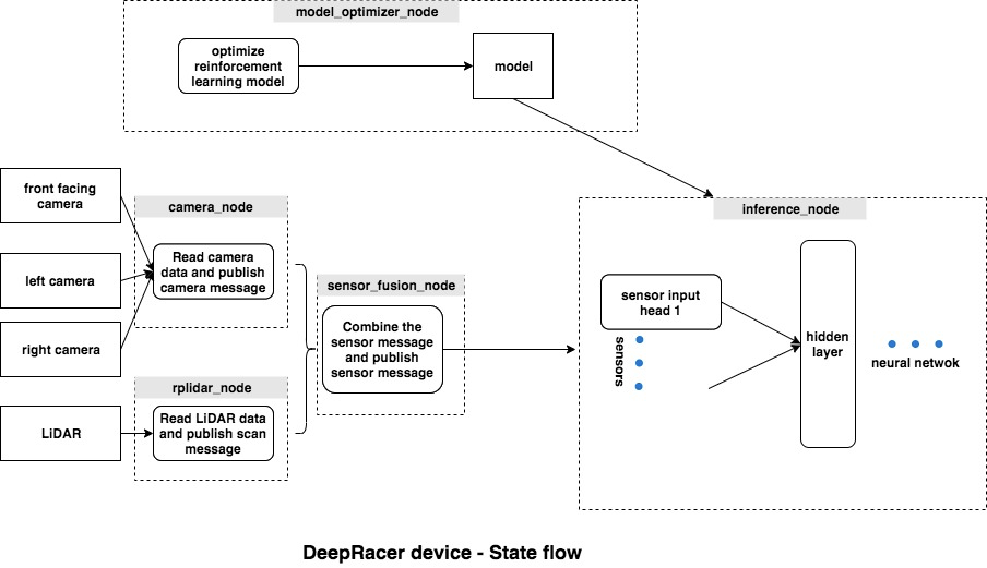
AWS DeepRacer. Allows exploration of RL. Simplifies the mapping of camera input to computer input, so one can focus more on the reward function and deep learning aspects. The car has a set of possible actions (change heading, change speed). The RL task is to predict the actions based on the inputs.
What are some of the strategies applied to winning DeepRacer ?
“DeepRacer: Educational Autonomous Racing Platform for Experimentation with Sim2Real Reinforcement Learning” – https://arxiv.org/pdf/1911.01562.pdf
DeepRacer uses RLLib which brings forth a key idea of encapsulating parallelism in the context of AI applications, as described in RLlib: Abstractions for Distributed Reinforcement Learning. RLLib is part of Ray, described in Ray: A Distributed Framework for Emerging AI Applications . Encapsulating parallelism means that individual components specify their own internal parallelism and resources requirements and can be used by other components without any knowledge of these. This allows a larger system to be built from modular components.
OpenAI Gym offers a suite of environments for developing and comparing RL algorithms. It emphasizes environments over agents, complexity over performance, knowledge sharing over competition. https://github.com/openai/gym , Open AI Gym paper. Here’s a code snippet from this paper of how they see an agent interact with the environments over 100 steps of a training episode.
ob0 = env.reset() # sample environment state, return first observation
a0 = agent.act(ob0) # agent chooses first action
ob1, rew0, done0, info0 = env.step(a0) # environment returns observation,
# reward, and boolean flag indicating if the episode is complete.
a1 = agent.act(ob1)
ob2, rew1, done1, info1 = env.step(a1)
...
a99 = agent.act(o99)
ob100, rew99, done99, info2 = env.step(a99)
# done99 == True => terminal
RL is not a fit for every problem. Alternative approaches with better explainability and determinism include behavior trees, vectorization/VectorNet, …
Deep learning is being applied to combinatorial optimization problems. A very intriguing talk by Anna Goldie discussed an application of RL to chip design that cuts down the time for layout optimization and which in turn enables optimizing of the chip design for a target software stack in simulation before the chip goes to production. Here’s a paper – graph placement methodology for fast chip design.
A snippet on how the research direction evolved to a learning problem.
“Chip floorplanning as a learning problem
The underlying problem is a high-dimensional contextual bandits problem but, as in prior work, we have chosen to reformulate it as a sequential Markov decision process (MDP), because this allows us to more easily incorporate the problem constraints as described below. Our MDP consists of four key elements: (1) States encode information about the partial placement, including the netlist (adjacency matrix), node features (width, height, type), edge features (number of connections), current node (macro) to be placed, and metadata of the netlist graph (routing allocations, total number of wires, macros and standard cell clusters). (2) Actions are all possible locations (grid cells of the chip canvas) onto which the current macro can be placed without violating any hard constraints on density or blockages. (3) State transitions define the probability distribution over next states, given a state and an action. (4) Rewards are 0 for all actions except the last action, where the reward is a negative weighted sum of proxy wirelength, congestion and density, as described below.
We train a policy (an RL agent) modelled by a neural network that, through repeated episodes (sequences of states, actions and rewards), learns to take actions that will maximize cumulative reward (see Fig. 1). We use proximal policy optimization (PPO) to update the parameters of the policy network, given the cumulative reward for each placement.”
Their diagram:
“An embedding layer encodes information about the netlist adjacency, node features and the current macro to be placed. The policy and value networks then output a probability distribution over available grid cells and an estimate of the expected reward for the current placement, respectively. id: identification number; fc: fullyconnected layer; de-conv: deconvolution layer”
“Fig. 1 | Overview of our method and training regimen.In each training iteration, the RL agent places macros one at a time (actions, states and rewards are denoted byai, si and ri, respectively). Once all macros are placed, the standard cells are placed using a force-directed method. The intermediate rewards are zero. The reward at the end of each iteration is calculated as a linear combination of the approximate wirelength, congestion and density, and is provided as feedback to the agent to optimize its parameters for the next iteration.”
PyTorch is an open source machine learning framework that is primarily used for building deep learning models. The framework is built on top of the Torch library and is implemented in Python, with support for C++ and CUDA.
The main C++ classes in PyTorch are:
Tensor: This is the core object in PyTorch and represents a multi-dimensional array. Tensors are the basic building blocks of a PyTorch model and are used to store and manipulate data.
Autograd: This is PyTorch’s automatic differentiation engine, which allows developers to compute gradients of tensors with respect to a loss function. The autograd module also provides a set of functions for computing gradients of complex functions.
nn.Module: This is a base class for all neural network modules in PyTorch. It provides a convenient way to define and organize layers of a neural network, as well as a set of useful methods for training and evaluating the model.
Optimizer: This is a class that implements various optimization algorithms, such as stochastic gradient descent (SGD), Adam, and Adagrad. The optimizer is used to update the parameters of a model during training.
DataLoader: This is a utility class that provides an efficient way to load and preprocess large datasets for training a model. The DataLoader class can be used to batch and shuffle data, as well as to apply various transformations to the data.
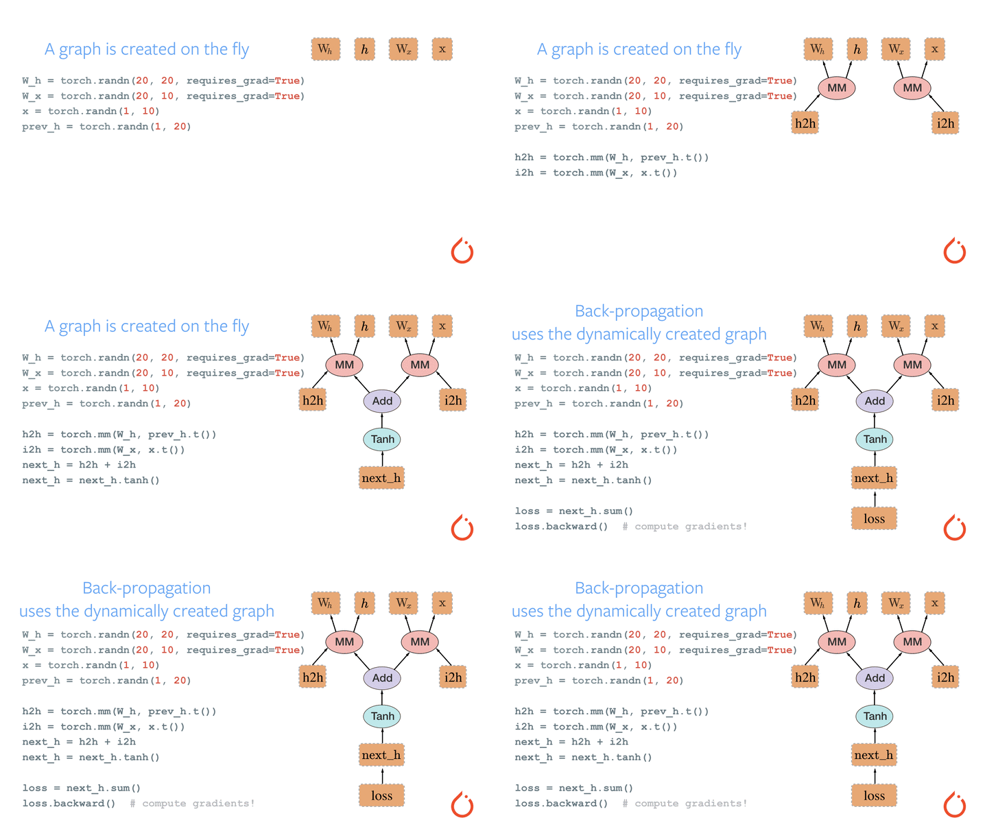
PyTorch’s autograd engine implements a variant of reverse-mode automatic differentiation, which is also known as backpropagation. This algorithm efficiently calculates the gradients of the output with respect to each input variable by traversing the computational graph in reverse order, propagating the gradients backwards through each operation using the chain rule.
In this paper – “DeepAR: Probabilistic Forecasting with Autoregressive Recurrent Networks”, the authors discuss a method for learning a global model from several individual time series.
Let’s break down some aspects of the approach and design.
“In probabilistic forecasting one is interested in the full predictive distribution, not just a single best realization, to be used in downstream decision making systems.”
The autoregressive model specifies that the output variable depends linearly on its own previous values and on a stochastic term (an imperfectly predictable term).
Recurrent Neural Network is used to refer to NNs with an infinite impulse response, and are used for speech recognition, handwriting recognition and such tasks involving sequences. https://en.wikipedia.org/wiki/Recurrent_neural_network
An LSTM or The Long Short-Term Memory (LSTM) is a type of RNN, that came about to solve a problem of vanishing gradients in previous RNN designs. An LSTM cell can process data sequentially and keep its hidden state through time.
A covariate is an independant random variable, with which the target random variable is assumed to have some covariance.
The approach has distinct features described in this snippet
“In addition to providing better forecast accuracy than previous methods, our approach has a number key advantages compared to classical approaches and other global methods: (i) As the model learns seasonal behavior and dependencies on given covariates across time series, minimal manual feature engineering is needed to capture complex, group-dependent behavior; (ii) DeepAR makes probabilistic forecasts in the form of Monte Carlo samples that can be used to compute consistent quantile estimates for all sub-ranges in the prediction horizon; (iii) By learning from similar items, our method is able to provide forecasts for items with little or no history at all, a case where traditional single-item forecasting methods fail; (vi) Our approach does not assume Gaussian noise, but can incorporate a wide range of likelihood functions, allowing the user to choose one that is appropriate for the statistical properties of the data. Points (i) and (iii) are what set DeepAR apart from classical forecasting approaches, while (ii) and (iv) pertain to producing accurate, calibrated forecast distributions learned from the historical behavior of all of the time series jointly, which is not addressed by other global methods (see Sec. 2). Such probabilistic forecasts are of crucial importance in many applications, as they—in contrast to point forecasts—enable optimal decision making under uncertainty by minimizing risk functions, i.e. expectations of some loss function under the forecast distribution.”
“A large machine learning job spans many nodes and runs most efficiently when it has access to all of the hardware resources on each node. This allows GPUs to cross-communicate directly using NVLink, or GPUs to directly communicate with the NIC using GPUDirect. So for many of our workloads, a single pod occupies the entire node. Any NUMA, CPU, or PCIE resource contention aren’t factors for scheduling. Bin-packing or fragmentation is not a common problem. Our current clusters have full bisection bandwidth, so we also don’t make any rack or network topology considerations. All of this means that, while we have many nodes, there’s relatively low strain on the scheduler.”
“We use iptables tagging on the host to track network resource usage per Namespace and pod. This lets researchers visualize their network usage patterns. In particular, since a lot of our experiments have distinct Internet and intra-pod communication patterns, it’s often useful to be able to investigate where any bottlenecks might be occurring.”
“the default setting for Fluentd’s and Datadog’s monitoring processes was to query the apiservers from every node in the cluster (for example, this issue which is now fixed). We simply changed these processes to be less aggressive with their polling, and load on the apiservers became stable again”
“ARP cache size increase..is particularly relevant in Kubernetes clusters since every pod has its own IP address which consumes space in the ARP cache”
“We use Kubernetes mainly as a batch scheduling system and rely on our autoscaler to dynamically scale up and down our cluster — this lets us significantly reduce costs for idle nodes, while still providing low latency while iterating rapidly. The default kube-scheduler policy is to spread out load evenly among nodes, but we want the opposite so that unused nodes can be terminated and also so that large pods can be scheduled quickly.”
Let’s take a disaster scenario where a system loses its data-in-transit (i.e. not yet persisted) at a certain point in time. and some time after this point, a recovery process kicks in, which restores the system back to normal functioning.
Recovery Point Objective refers to the amount of tolerable data loss measured in time. It can be measured in time based on the fact that it is in-transit data of a certain max velocity, so bounding the time bounds the amount of data that can be lost. This time figure, the RPO, is used to determine how frequently the data must be persisted and replicated. An RPO of 10 minutes implies the data must be backed up every 10 minutes. If there’s a crash the system can be restored to a point not more than 10 minutes prior to the time of crash. RPO determines frequency of backups, snapshots or transaction logs.
Recovery Time Objective refers to the amount of time required to restore a system to normal behavior after a disaster has happened. This includes restoration of all infrastructure components that provide a service, not just the restoration of data.
Lower RPO/RTO is higher cost.
Matrix of RPO – high/low vs RTO – high/low can be used to categorize applications.
Low RPO, Low RTO. Critical online application like a storefront.
Low RPO, High RTO. Data sensitive application but not online, like analytics.
High RPO, Low RTO. Redundantly available data or no data. Compute clusters that are highly available.
High RPO, High RPO. Non-prod systems – dev/test/qa ?
Amount of acceptable data loss <= App (data?) criticality. One can expect a pyramid of apps – large number with less criticality, small number with high criticality
Repeatability. Backup and recovery procedures. Must be written. Must be tested. Automation.
HA/DR spectrum of solutions:
Backups, save transaction logs
Snapshots
Replication – synchronous, asynchronous
Storage only vs in-memory as well. Application level crash consistency of backups.
Multiple AZs
Hybrid
Tech: S3 versioning and DDB streams, Global tables.
Rules of thumb:
test full recovery regularly, at least once an year.
Keep at least 3 copies of data in at least 2 media types, and at least one off-site backup.
Related terms: RPA and RTA
3 types of disasters.
Natural disaster – e.g. floods, earthquakes, fire
Technical failure – e.g. loss of power, cable pulled
Human error – e.g. delete all files as admin
Replication – works for first two. Continuous snapshots/backup/versioning – for the last one. Replication will just delete the data on both sides. Need the ability to go back in time and restore data.
Cost – how to optimize cost of infrastructure and its maintenance.
Which region to choose ? Key considerations: What types of disasters are the concern (Risk). How much proximity is needed to end-customers and to primary region (Performance). What’s the cost of the region (Cost) ?
The threat detection problem, use-cases and scale.
It’s important to focus on and build the data platform first else one can get siloed into narrow set of addressable use-cases.
we want to detect attacks,
contextualize the attacks
determine root cause of an attack,
determine what the scope of the incident might be
determine what we need to contain it
Diverse threats require diverse data sets
the Threat signal can be concentrated or spread in time
Keylines visualization library is used to build a visualization of detection, contextualization, containment
Streaming is a simple pattern that takes us very far for detection
Streams are left-joined with context and filtered or inner-joined with indicators
Can do a lot with this but not everything
Graphs are key. Graphs at scale are super hard.
Enabling triage and containment with search and query
to triage the detection, it comes down to search and query.
ETM does 3.5million records/sec. 100TB of data a day. 300B events a day.
11 trillion rows, 0.5PB of data.
Ingestion architecture – tries to solve all these problems and balance issues.
data comes into s3 in a consistent json wrapper
there’s a single ETL job that takes all the data and writes it into a single staging table which is partitioned by date and event-type, has a long retention
table is optimized to stream new data in and stream data out of, but can be queried as well. you can actually go and query it using sql function
highest value data – we write parsers, we have discrete parsing streams and put them into a common schema and put it into separate delta tables. well parsed, well structured.
use optimizations from delta, z-odering.. to index over columns that are common predicates. search by IP address, domain names – those are what we order by
indexing and z-ordering – take advantage of data skipping
sometimes we parser code gets messed up.
single staging table.. is great . we just let the fixed parser run forward, we have all the data corrected, then we are back-corrected. don’t have to repackage code and run as a batch job. we literally just fix code and run it in the same model that’s it.
off of these refined tables or parsed data sets, this is where the detection comes in.
we have a number of detection streams in batches, that do the logic and analysis. facet-faced or statistical.
alerts that come out of this go to their own alert table. goes to delta again. long retection, consistent schema. another streaming job then does de-duplication and whitelisting and writes out alerts to our alert management system. we durably store all the alerts, whether or not de-duped/whitelisted
allows us to go back and fix things if things are not quite correct, accidentally.
all this gives us operational sanity, and a nice feedback loop
Thanks to z-ordering, it can go from scanning 500TB to 36TB.
average case is searching over weeks or months. it makes it usable for ad-hoc refinements.
simple, unified platform.
Michael: Demo on interactive queries over months of data
first attempt is sql SELECT on raw data. takes too long, cancelled. second attempt uses HMS, still too long, cancelled. why is this so hard ?
observation: every data problem is actually two problems 1) data engineering and 2) data science. most projects fail on step 1.
doing it with delta – the following command takes 17s and fires off spark job to put the data in a common schema.
CREATE TABLE connections USING delta AS SELECT * from json.'/data/connections'
then
SELECT * FROM connections WHERE dest_port = 666
this is great to query the historical data quickly.. however batch alone is not going to cut it as we may have attacks going on right now. but delta plugs into streaming as well:
INSERT INTO connections SELECT * from kafkaStream
Now we’ve Indexed both batch and streaming data.
We can run a python netviz command to visualize the connections.
Smithy is an Apache-2.0 licensed, protocol-agnostic IDL for defining APIs, generating clients, servers and documentation. https://github.com/awslabs/smithy
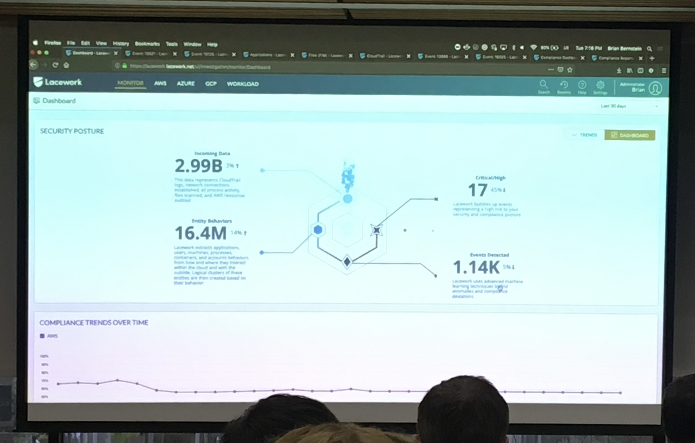
Lacework Polygraph is a Host based IDS for cloud workloads. It provides a graphical view of who did what on which system, reducing the time for root cause analysis for anomalies in system behaviors. It can analyze workloads on AWS, Azure and GCP.
It installs a lightweight agent on each target system which aggregates information from processes running on the system into a centralized customer specific (MT) data warehouse (Snowflake on AWS) and then analyzes the information using machine learning to generate behavioral profiles and then looks for anomalies from the baseline profile. The design allows automating analysis of common attack scenarios using ssh, privilege changes, unauthorized access to files.
The host based model gives detailed process information such as which process talked to which other and over what api. This info is not available to a network IDS. The behavior profiles reduce the false positive rates. The graphical view is useful to drill down into incidents.
It does not have an intrusion prevention (IPS) functionality. False positives on an IPS could block network/host access and negatively affect the system being protected, so it’s a harder problem.
Cloud based network isolation tools like Aviatrix might make IPS scenarios feasible by limiting the effect of an IPS.
Iptables is a Linux-based firewall utility that allows system administrators to configure rules and filters for network traffic. It works by examining each packet that passes through the system and making decisions based on rules defined by the administrator.
In the context of iptables, tables are organizational units that contain chains and rules. There are five built-in tables in iptables:
filter – This is the default table and is used for packet filtering.
nat – This table is used for network address translation (NAT).
mangle – This table is used for specialized packet alteration.
raw – This table is used for configuring exemptions from connection tracking in combination with the NOTRACK target.
security – This table is used for Mandatory Access Control (MAC) networking rules.
In iptables, a chain is a sequence of rules that are applied to each packet passing through a particular table. Each table contains several built-in chains, and these chains can also have user-defined chains.
Each table contains several built-in chains and can also have user-defined chains. The chains contain rules that are used to determine what happens to packets as they pass through the firewall.
The name “chain” comes from the way that iptables processes packets. When a packet arrives at the firewall, it is first matched against the rules in the PREROUTING chain. If the packet matches a rule in that chain, it is processed according to the action specified in the rule. If the packet is not matched by any rules in the PREROUTING chain, it is then passed to the INPUT chain, where it is again matched against each rule.
This process continues through the FORWARD, OUTPUT, and POSTROUTING chains until the packet is either accepted, rejected, or dropped. Because each chain is a sequence of rules that are processed in order, it is called a “chain.”
In iptables, there are five types of chains. Not all of the five chains are present in all the tables. The PREROUTING, INPUT, and FORWARD chains are present in the “filter” and “raw” tables. The OUTPUT and POSTROUTING chains are present in the “filter”, “nat”, and “mangle” tables.
The “security” table, which is used for Mandatory Access Control (MAC) networking rules, does not have the PREROUTING, POSTROUTING, or OUTPUT chains. Instead, it has inbound and outbound chains for each network interface.
Each of these chains has a default policy that can be set to either ACCEPT, DROP, or REJECT. ACCEPT means that the packet is allowed through, DROP means that the packet is silently discarded, and REJECT means that the packet is discarded and the sender is notified.
System administrators can create custom rules that match specific criteria, such as the source or destination IP address, the protocol used, or the port number.
“mangle” is a table that is used to alter or mark packets in various ways. The mangle table provides a way to modify packet headers in ways that other tables cannot, such as changing the Time To Live (TTL) value or the Type of Service (TOS) field.
Before I forget it’s name, BaseCoin is a project that attempts to stabilize a cryptocurrency, so it does not have wild fluctuations.
Regular (Fiat) currencies are actively managed by Federal banks to be stable and are also stabilized by being the default currency for labor negotiations, employment contracts, retirement accounts etc which are slow moving changes.
https://en.wikipedia.org/wiki/Stablecoin notes that Basis coin failed. It also makes a distinction between fiat-backed stablecoins and cryptocurrency backed stablecoin. In the latter the stabilizing algo works on chain.