Tag: machine learning

Absolute Zero: zero reliance on external data to improve model reasoning

Imagine you want to train a large language model to get really good at solving tough problems—things like math puzzles or writing correct code. Usually, the way people do this is by giving the model lots of practice questions written by humans. These are called human-curated tasks: real people come up with the problems and answers, like “Write a program to reverse a string” or “What’s the derivative of x²?”. The model practices on these problem-solution pairs, and then reinforcement learning (RL) or reinforcement learning with verifiable rewards (RLVR) can be used to improve how it reasons.

But as models get bigger and smarter, collecting enough high-quality problems from humans becomes expensive, slow, and limiting. If the model might one day surpass most humans, why should humans be the bottleneck?

That’s where this paper’s idea, called Absolute Zero, comes in. Instead of relying on people to write problems, the model creates its own. One part of the model plays the “teacher,” proposing new tasks, and another part plays the “student,” trying to solve them. Because the environment is code, the answers can be automatically checked just by running the program—so no human needs to grade them.

The model learns three kinds of reasoning:

  • Deduction: given a program and input, figure out the output.
  • Abduction: given a program and an output, figure out the input.
  • Induction: given some examples, figure out the program that works in general.

The system rewards the student for solving problems correctly, and the teacher for coming up with problems that are just the right difficulty—not too easy, not impossible.

The result is that training only on these self-made coding tasks made the model better at math. On standard benchmarks, it matched or even beat other models that were trained with large sets of human-written problems. Bigger models improved even more, and “coder” models (already good at programming) saw the biggest gains. The model even started showing “scratch-pad” style reasoning on its own, writing little notes or plans before coding—without being told to.

In short, the key insight is this: you don’t necessarily need humans to write all the practice problems anymore. If you have a way to automatically check answers, a model can bootstrap itself, creating and solving its own challenges, and still learn to reason across domains.

The authors do warn that there are challenges—like making sure tasks stay diverse, keeping the system safe, and managing the heavy compute costs—but the big takeaway is that self-play with verifiable rewards could be a new path to building smarter, more independent reasoning systems.

There’s no “exam” in the usual sense for the students – the system builds a feedback loop between the teacher (proposer) and the student (solver).

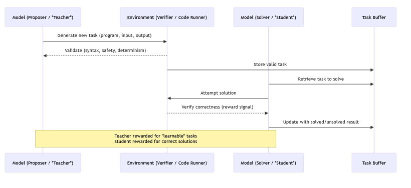
Here’s how it works step by step:

1. Teacher proposes a task

The proposer (teacher model) generates a new program + input/output pair (a problem).

Example: “Write a function that finds prime numbers up to N.”

2. Environment checks validity

The environment (code runner) ensures the task is valid: it runs, is safe, deterministic, etc.

If valid, it gets stored in a task buffer.

3. Student attempts the task

The solver (student model) pulls the task and tries to solve it.

The environment executes the student’s answer and checks correctness.

4. Rewards reflect difficulty

If the student always solves a task → it’s too easy → proposer gets low reward.

If the student never solves a task → it’s too hard → proposer also gets low reward.

If the student solves it sometimes → it’s “learnable” → proposer gets high reward.

So the proposer doesn’t “know” in advance how good the student is. Instead, it learns over time:

Tasks that end up being useful for training (medium difficulty) get reinforced.

Tasks that are too trivial or impossible fade out because they bring no proposer reward.

The proposer is like a coach who experiments with new drills, and the student’s performance on them acts as the exam. Over time, the teacher learns what kinds of problems best stretch the student without breaking them.

RDMA, Infiniband, RoCE, CXL : High-Performance Networking Technologies for AI

As the demand for high-performance computing (HPC) and artificial intelligence (AI) continues to grow, networking technologies have become critical to ensuring the scalability and efficiency of modern data centers. Among these, RDMA, InfiniBand, RoCE, and the emerging CXL standard stand out as transformative technologies, each addressing unique challenges. Here’s a brief overview of these key technologies, trends, and future.

Remote Direct Memory Access (RDMA) was developed in response to the increasing need for low-latency, high-bandwidth data movement in distributed computing environments. RDMA was driven by a collaboration of major tech companies to address the limitations of traditional networking models. Some key players in RDMA’s early development include:

  • Compaq, IBM, and Intel:
    • Developed the initial RDMA architecture to improve networking efficiency, particularly in storage and high-performance computing.
  • Mellanox Technologies:
    • One of the first companies to commercialize RDMA with its InfiniBand solutions, allowing ultra-low latency communication.
  • Microsoft & Networking Industry:
    • Developed iWARP (RDMA over TCP/IP) to integrate RDMA into Ethernet-based networks.
  • InfiniBand Trade Association (IBTA):
    • Founded in 1999 by Compaq, Dell, Hewlett-Packard, IBM, Intel, Microsoft, and Sun Microsystems to standardize high-performance networking, including RDMA capabilities.

Before RDMA, networking relied on CPU-intensive packet processing, which created performance bottlenecks in data-intensive applications. The traditional TCP/IP stack required multiple CPU interrupts, context switches, and memory copies, leading to high latency and inefficiency.

RDMA Was Developed to Solve These Challenges:

  1. Eliminate CPU Bottlenecks:
    • Traditional networking required CPU cycles for data movement, slowing down high-speed applications.
    • RDMA bypasses the OS kernel and CPU, reducing overhead.
  2. Enable High-Speed, Low-Latency Communication:
    • Needed for HPC (High-Performance Computing), AI training, and databases.
    • Reduces communication latency to below 1 microsecond.
  3. Improve Scalability for Distributed Systems:
    • Large-scale data centers and supercomputers require fast inter-node communication.
    • RDMA enables efficient parallel computing across thousands of nodes.
  4. Optimize Storage and Networking:
    • Technologies like NVMe over Fabrics (NVMe-oF) use RDMA for ultra-fast storage access.
    • RDMA dramatically speeds up databases and cloud storage, reducing I/O latency.

Evolution and Implementations of RDMA

RDMA has evolved into different implementations, each suited for different networking environments:

RDMA VariantTransport ProtocolUse Case
InfiniBandNative InfiniBand transportHPC, AI training, supercomputing
RoCE (RDMA over Converged Ethernet)Ethernet (Layer 2/3)Cloud data centers, AI inference
iWARPTCP/IPEnterprise storage, cloud computing

RDMA’s Impact on Modern Computing

Today, RDMA is a core technology in AI, cloud computing, and high-speed storage. It enables:

  • Massive parallelism in AI training (e.g., NVIDIA DGX, GPT models).
  • Faster database transactions (e.g., Microsoft SQL Server, Oracle).
  • Low-latency cloud networking (used by Azure, AWS, Google Cloud).

InfiniBand: InfiniBand is a high-performance networking technology designed for low-latency, high-bandwidth communication. Primarily used in HPC and AI training clusters, InfiniBand supports features like Remote Direct Memory Access (RDMA), enabling direct memory-to-memory data transfers with minimal CPU involvement. Its scalable architecture makes it ideal for distributed workloads, offering latencies as low as 0.5 microseconds and bandwidths up to 400 Gbps (NDR).

RDMA over Converged Ethernet (RoCE): RoCE extends RDMA capabilities over Ethernet networks, bridging the gap between the performance of InfiniBand and the ubiquity of Ethernet. By leveraging standard Ethernet infrastructure with lossless configurations, RoCE delivers efficient communication for data centers that prioritize compatibility and cost. However, it typically exhibits slightly higher latencies (5-10 microseconds) compared to InfiniBand.

Compute Express Link (CXL): CXL is a new interconnect standard designed to provide low-latency, high-bandwidth communication between processors, accelerators, and memory devices within a single node. By leveraging PCIe infrastructure, CXL supports memory pooling, coherent data sharing, and dynamic resource allocation, addressing the growing complexity of heterogeneous compute environments

Key Technology Trends
  1. AI Training Driving High-Bandwidth Demand:
    • Training large-scale AI models requires massive data exchange between GPUs, CPUs, and memory. InfiniBand remains the leader in this domain due to its ultra-low latency and scalability, but RoCE is increasingly adopted in cost-sensitive deployments.
  2. Distributed Inference and Edge AI:
    • While inference typically has lower communication demands, distributed inference pipelines and edge AI are pushing for efficient interconnects. RoCE’s compatibility with Ethernet makes it a strong candidate in these scenarios.
  3. Memory-Centric Architectures:
    • With CXL’s focus on memory pooling and coherent memory sharing, the future of data centers may see significant convergence around flexible, node-level resource allocation. This complements, rather than competes with, network-level technologies like InfiniBand and RoCE.
  4. Interconnect Ecosystem Integration:
    • NVIDIA’s integration of InfiniBand with its GPUs and DPUs highlights the trend of tightly coupled compute and networking stacks. Similarly, innovations in RoCE and Ethernet SmartNICs are bringing RDMA capabilities closer to mainstream data centers.
Extrapolating to the future
  • Convergence of Standards: As workloads diversify, data centers may adopt hybrid approaches, combining InfiniBand for training clusters, RoCE for distributed inference, and CXL for intra-node memory coherence. Seamless interoperability between these standards will be ideal.
  • AI-Centric Network Evolution: The growing dominance of AI workloads will push networking technologies toward even lower latencies and higher bandwidths, with InfiniBand and RoCE leading the charge.
  • Rise of Heterogeneous Compute: CXL’s potential to unify memory access across CPUs, GPUs, and accelerators aligns with the industry’s shift toward heterogeneous compute, enabling efficient resource utilization and scalability.
  • Cloud-Driven Innovations: As hyperscalers like AWS, Google, and Azure integrate these technologies into their offerings, cost-efficient, scalable solutions like RoCE and CXL may become more widespread, complementing specialized InfiniBand deployments.

Direct Preference Optimization (DPO) vs RLHF/PPO (Reinforcement Learning with Human Feedback, Proximal Policy Optimization)

The paper “Direct Preference Optimization: Your Language Model is Secretly a Reward Model” introduces Direct Preference Optimization (DPO), an algorithm for fine-tuning language models to align with human preferences without the need for complex reinforcement learning procedures. This simplifies Reinforcement Learning with Human Feedback (RLHF) by not requiring a time consuming human feedback loop in training of the model.

Directly Modified Reward Function : DPO uses human preferences to directly modify the reward function, employing a classification loss to align the model outputs with these preferences. Rather than relying solely on reward signals from the environment, it leverages comparisons or preferences between different trajectories to guide the learning process. The agent is provided with pairs of trajectories along with a preference indicating which trajectory is preferred. This preference data is used to train the policy. The task of predicting preferences can be framed as a binary classification problem. For a given pair of trajectories the model needs to predict which path is preferred. The classification loss then measures the discrepancy between the predicted and actual preferences. A common choice for this kind of binary classification is the binary cross-entropy loss. The overall training objective in DPO involves minimizing the classification loss across all pairs of trajectories in the dataset, which encourages the policy to produce trajectories that align with the observed preferences.

RLHF and Proximal Policy Optimization: RLHF trains a reward model using PPO and data gathered on human preferences that is labeled by humans. These RLHF steps are shown in the diagram below, from the RLHF paper. PPO indirectly learns the reward function through interactions with the environment and optimizes the policy to maximize this reward, using a reinforcement learning framework. The policy here is a mapping from states to a probability distribution over actions.

So Direct Preference Optimization (DPO) modifies the reward function using human preference data. Here is a high-level overview of the equations used:

  1. Preference Model:
    • Let θ be the parameters of the model.
    • Let τ1​ and τ2​ be two trajectories (or outputs) being compared.
    • The preference model P(τ1≻τ2∣θ)  indicates the probability that humans prefer τ1​ over τ2​.
  2. Logistic Function for Preferences:
    • The preference probability is modeled using a logistic function:P(τ1≻τ2∣θ)=exp⁡(R(τ1∣θ)) / ( exp⁡(R(τ1∣θ)) + exp⁡(R(τ2∣θ)) )
    • R(τ∣θ) is the reward function for trajectory τ.
  3. Loss Function:
    • The loss function L(θ) is defined as the negative log-likelihood of the human preferences:L(θ)=−∑(τ1,τ2)∈D log⁡ P(τ1≻τ2∣θ)
    • D is the dataset of human preference comparisons.
  4. Optimization:
    • The model parameters θ are optimized by minimizing the loss function L(θ)

GPU kernel functions for deep learning

This article attempts to outline GPU Kernel Functions and how they are supported in TensorFlow, PyTorch, and OpenAI Triton. GPU Kernel Functions are specialized functions executed on an Nvidia Graphics Processing Unit. These functions play a key role in for parallel and accelerated computing such as tensor matrix operations used in deep learning.

GPU kernel functions for operations commonly used in deep learning include:

  1. Element-wise operations: TensorFlow provides GPU kernels for element-wise operations such as addition, subtraction, multiplication, and division, enabling efficient computation on arrays or tensors.
  2. Matrix operations: GPU kernels in TensorFlow optimize matrix operations like matrix multiplication, matrix addition, and matrix transpose, which are fundamental in many deep learning models.
  3. Convolutional operations: TensorFlow implements GPU kernels for convolutional operations, which are essential for tasks like image recognition and computer vision.
  4. Reduction operations: TensorFlow provides GPU kernels for reduction operations like summation, mean, maximum, and minimum, allowing efficient computation over large arrays or tensors.
  5. Activation functions: GPU kernels are implemented for common activation functions used in deep learning, such as ReLU (Rectified Linear Unit), sigmoid, and tanh.
  6. Pooling operations: TensorFlow’s GPU kernels optimize pooling operations like max pooling and average pooling, commonly used in convolutional neural networks (CNNs).
  7. Recurrent operations: TensorFlow provides GPU kernels for recurrent operations like LSTM (Long Short-Term Memory) and GRU (Gated Recurrent Unit), which are widely used in sequence-based models.

TensorFlow optimizes the execution of operations within a computation graph. When operations can be executed on a GPU, TensorFlow translates the high-level operations into CUDA calls that invoke the corresponding GPU kernels.

PyTorch is another popular open-source deep learning framework that provides a high-level programming interface for building and training machine learning models.

PyTorch differs from TensorFlow in a few ways:

  1. Dynamic Computational Graph: PyTorch uses a dynamic computational graph approach, whereas TensorFlow uses a static computational graph. This means that in PyTorch, the computational graph is constructed and executed on the fly as the code is executed, allowing for more flexibility and dynamic behavior during model training and inference.
  2. Imperative Programming: PyTorch follows an imperative programming style, which allows users to write code that is more intuitive and resembles standard Python programming. This makes it easier to understand and debug the code, as well as experiment with different model architectures and algorithms.
  3. Autograd: PyTorch’s autograd system allows automatic differentiation, which enables computing gradients for model parameters. This makes it easier to implement and train complex models, as users don’t have to manually compute gradients. TensorFlow, on the other hand, uses a static graph approach where gradients need to be explicitly defined and computed.
  4. TorchScript: PyTorch provides a feature called TorchScript, which allows models to be serialized and optimized for deployment in production environments. TorchScript enables efficient execution of PyTorch models on various platforms, including GPUs, CPUs, and mobile devices.

Like TensorFlow, PyTorch also implements GPU kernel functions for efficient computation on GPUs. It implements optimized GPU kernels similar to TensorFlow.

So while both TensorFlow and PyTorch provide GPU kernel function abstractions, their underlying computational graph models and programming styles differ, bringing their own unique advantages and trade-offs.

OpenAI Triton is a programming framework developed by OpenAI for building and deploying large-scale machine learning models efficiently. It leverages TensorFlow as its backend, supporting a wide range of models including deep learning and traditional algorithms. Triton offers tools for distributed computing, automated hyperparameter tuning, and model serving. It simplifies model deployment and management, making it suitable for both research and production environments. Triton abstracts away the need for users to write low-level GPU kernel functions by using TensorFlow’s optimized GPU operations implemented with CUDA, NVIDIA’s parallel computing platform. This approach allows developers to focus on defining high-level machine learning models without worrying about GPU optimization details.

It’s worth noting that Triton is built on top of TensorFlow, which supports alternative GPU acceleration libraries through backend integrations, and this enables Triton to leverage these alternatives to CUDA. One such alternative to CUDA is ROCm (Radeon Open Compute platform), developed by AMD. ROCm is an open-source GPU computing platform that provides support for AMD GPUs. TensorFlow has been working on integrating with ROCm, allowing it to utilize AMD GPUs for deep learning computations. As Triton relies on TensorFlow, it can benefit from this integration to support AMD GPUs through ROCm.

TorchScript for Model Optimization and Model Serving

TorchScript is an intermediate representation of a PyTorch model that can be optimized and run in a non-Python environment, making the PyTorch model suitable for deployment. It is part of the PyTorch ecosystem (Intro_to_TorchScript_tutorial.html , TorchScript JIT.html ).

Why is TorchScript needed ? Python while excellent for ML model development ( interpreted, REPL, simplicity, integration with number of ML libraries), also has characteristics that make it less suitable for model production deployments. These characteristics include interpretation overheads, complex dependency management, high memory/CPU overheads and the lack of easy integration with native technologies such as C++ for high performance and for embedded systems. TorchScript provides tools for optimizations such as operator fusion and static graph analysis which can improve the efficiency and performance during inference. Optimizing the models is crucial for embedded systems with limited resources.

PyTorch had introduced eager/dynamic execution, which had the advantage of faster user feedback but the disadvantage of not having as many optimizations as were possible in static approaches as in Tensorflow.

A blog on Key points to grasp about TorchScript – https://medium.com/@hihuaweizhu/key-points-to-grasp-for-torchscript-beginners-c02cf94aaa50, makes several good points, including that TorchScript is a subset of PyTorch and consists of statically typed variables.

A discussion between eager mode and script mode at https://towardsdatascience.com/pytorch-jit-and-torchscript-c2a77bac0fff suggests the benefit of TorchScript is more about dev/production (versus training/inference), with the production version requiring performance optimizations and portability. Quote: “With TorchScript, PyTorch aims to create a unified framework from research to production. TorchScript will take your PyTorch modules as input and convert them into a production-friendly format.

NVIDIA uses TorchScript to facilitate the deployment and optimization of PyTorch models within their ecosystem. The Torchscript models are compiled to TensorRT, the Nvidia runtime .

AWS ML software stack, Neuron, supports tracing in torchscript. https://awsdocs-neuron.readthedocs-hosted.com/en/latest/frameworks/torch/torch-neuronx/api-reference-guide/inference/api-torch-neuronx-trace.html . https://pytorch.org/docs/master/generated/torch.jit.trace.html#torch.jit.trace . An example of a neuron sdk trace for pytorch – https://github.com/aws-neuron/aws-neuron-sdk/issues/371 .

PyTorch/XLA is another project that integrates with Google XLA compiler to enable running PyTorch models on Google TPUs.

GraphCore produces hardware for deep learning called a GraphCore Intelligence Processing Unit (IPU). The primary software framework provided by GraphCore to execute machine learning models on their IPUs is Poplar. It allows running models from TensorFlow and PyTorch. Poplar optimizes computations for the unique architecture of GraphCore’s IPUs. This includes optimizations for memory bandwidth, parallel processing, and other hardware-specific features.

Deep Reinforcement Learning key papers

Reinforcement Learning (RL) combined with Deep Learning has been termed Deep Reinforcement Learning (DRL). Deep learning provides function approximation techniques that can handle large and complex state and/or action spaces, making it possible to tackle problems that were infeasible with traditional RL techniques. This line of research led to transformers and LLMs. Here’s a brief timeline of key insights and breakthroughs in Deep Reinforcement Learning over the past decade:

1. 2013Playing Atari with Deep Reinforcement Learning:
  • Organization: DeepMind
  • Breakthrough: This was perhaps the first major work that combined deep learning with Q-learning, resulting in a Deep Q-Network (DQN). The DQN was able to play several Atari 2600 games at or above human-level performance.
  • Key Insights: Experience replay and fixed Q-targets were used to stabilize learning. The experience replay helped in breaking the temporal correlations, and fixed Q-targets reduced the moving target problem in Q-learning.
2. 2015Human-level control through deep reinforcement learning:
  • Organization: DeepMind
  • Breakthrough: An extension of the 2013 DQN work, this presented a more robust DQN that achieved human-level performance across a broad range of Atari games.
  • Key Insights: Further stabilization and scaling of DQNs.
3. 2015Continuous control with deep reinforcement learning (DDPG):
  • Organization: DeepMind
  • Breakthrough: Introduced the Deep Deterministic Policy Gradient (DDPG) algorithm for continuous action spaces.
  • Key Insights: It utilized actor-critic architecture where the actor produces a deterministic policy, and the critic evaluates it. The Ornstein-Uhlenbeck process was used to add exploration noise.
4. 2016Asynchronous Methods for Deep Reinforcement Learning (A3C):
  • Organization: DeepMind
  • Breakthrough: Introduced the Asynchronous Advantage Actor-Critic (A3C) algorithm which combined the actor-critic approach with asynchronous updates.
  • Key Insights: Multiple agents, each with its own set of model parameters, explored different parts of the environment simultaneously, leading to faster and more robust policy learning. The asynchronous nature also helped in stabilizing learning.
5. 2017Proximal Policy Optimization (PPO):
  • Organization: OpenAI
  • Breakthrough: Introduced a simpler and more robust method for policy gradient optimization, making training more stable.
  • Key Insights: PPO constrains the policy updates to ensure the new policy isn’t too different from the old policy, thereby avoiding extreme policy updates that can destabilize training. PPO balances the benefits of both Policy Gradient methods (link) and Trust Region Policy Optimization methods (TRPO link). PPO achieves this by using a clipped surrogate objective that prevents large updates during training, enhancing stability and performance. In the context ofPPO, the term “surrogate objective” refers to an approximation used in place of the actual objective function during optimization. This surrogate function is easier to optimize and ensures more stable and reliable updates to the policy. The clip function ensures that the probability ratiodoes not deviate too far from 1 by clipping it to the range [1−ϵ,1+ϵ][1−ϵ,1+ϵ]. This prevents excessively large policy updates.
6. 2018Soft Actor-Critic (SAC):
  • Organization: UC Berkeley
  • Breakthrough: SAC is an off-policy actor-critic deep RL algorithm based on the maximum entropy RL framework.
  • Key Insights: SAC seeks policies that maximize both expected return and entropy, leading to more exploration, smoother policy updates, and generally better performance on continuous control tasks.
7. 2019 and beyond:

Subsequent years have seen the evolution of these methods and the introduction of new algorithms, improvements in sample efficiency, stability, and scalability. Also, there has been a focus on:

  • Transfer Learning: Using pre-trained models to improve sample efficiency in RL.
  • Meta-learning: Training agents that can quickly adapt to new tasks.
  • Model-based RL: Incorporating learned models of the environment dynamics to improve sample efficiency and policy learning.

Accuracy vs Recall vs Precision vs F1 in Machine Learning

We want to walk through some common metrics in classification problems – such as accuracy, precision and recall – to get a feel for when to use which metric. Say we are looking for a needle in a haystack. There are very few needles in a large haystack full of straws. An automated machine is sifting through the objects in the haystack and predicting for each object whether it is a straw or a needle. A reasonable predictor will predict a small number of objects as needles and a large number as straws. A prediction has two attributes – positive/negative and accurate/inaccurate.

Positive Prediction: the object at hand is predicted to be the needle. A small number.

Negative Prediction: the object at hand is predicted not to be a needle. A large number.

True_Positive: of the total number of predictions, the number of predictions that were positive and correct. Correctly predicted Positives (needles). A small number.

True_Negative: of the total number of predictions, the number of predictions that were negative and correct. Correctly predicted Negatives (straws). A large number.

False_Positive: of the total number of predictions, the number of predictions that are positive but the prediction is incorrect. Incorrectly predicted Positives (straw predicted as needle). Could be large as the number of straws is large, but assuming the total number of predicted needles is small, this is less than or equal to predicted needles, hence small.

False_Negative: of the total number of predictions, the number of predictions that are negative but the prediction is incorrect. Incorrectly predicted Negatives (needle predicted as straw). Is this a large number ? It is unknown – this class is not large just because the class of negatives is large – it depends on the predictor and a “reasonable” predictor which predicts most objects as straws, could also predict many needles as straws. This is less than or equal to the total number of needles, hence small.

Predicted_Positives = True_Positives + False_Positives = Total number of objects predicted as needles.

Actual Positives = Actual number of needles, which is independant of the number of predictions either way, however Actual Positives = True Positives + False Negatives.

Accuracy = nCorrect _Predictons/nTotal_Predictions=(nTrue_Positives+nTrue_Negatives) / (nPredicted_Positives +nPredicted_Negatives) .   # the reasonable assumption above is equivalent to a high accuracy. Most predictions will be hay, and be correct in this simply because of the skewed distribution. This does not shed light on FP or FN.

Precision = nTrue_Positives / nPredicted_Positives    # correctly_identified_needles/predicted_needles;  this sheds light on FP; Precision = 1 => FP=0 => all predictions of needles are in fact needles; a precision less than 1 means we got a bunch of hay with the needles – gives hope that with further sifting the hay can be removed.  Precision is also called Specificity and quantifies the absence of False Positives or incorrect diagnoses.

Recall = nTrue_Positives / nActual_Positives  = TP/(TP+FN)# correctly_identified_needles/all_needles; this sheds light on FN; Recall = 1 => FN = 0; a recall less than 1 is awful as some needles are left out in the sifting process. Recall is also called Sensitivity .

Precision > Recall => FN is higher than FP

Precision < Recall => FN is lower than FP

If at least one needle is correctly identified as a needle, both precision and recall will be positive; if zero needles are correctly identified, both precision and recall are zero.

F1 Score is the harmonic mean of Precision and Recall.  1/F1 = 1/2(1/P + 1/R) . F1=2PR/(P+R) .  F1=0 if P=0 or R=0. F1=1 if P=1 and R=1.

ROC/AUC rely on Recall (=TP/TP+FN) and another metric False Positive Rate defined as FP/(FP+TN)  = hay_falsely_identified_as_needles/total_hay . As TN >> FP, this should be close to zero and does not appear to be a useful metric in the context of needles in a haystack; as are ROC/AuC . The denominators are different in Recall and FPR, total needles and total hay respectively.

There’s a bit of semantic confusion when saying True Positive or False Positive. These shorthands can be interpreted as- it was known that an instance was a Positive and a label of True or False was applied to that instance. But what we mean is that it was not known whether the instance was a Positive, and that a determination was made that it was a Positive and this determination was later found to be correct (True) or incorrect (False). Mentally replace True/False with ‘Correct/Incorrectly identified as’ to remove this confusion.

Normalization: scale of 0-1, or unit norm; useful for dot products when calculating similarity.

Standardization: zero mean, divided by standard deviation; useful in neural network/classifier inputs

Regularization: used to reduce sensitivity to certain features. Uses regression. L1: Lasso regression L2: Ridge regression

Confusion matrix: holds number of predicted values vs known truth. Square matrix with size n equal to number of categories.

Bias, Variance and their tradeoff. we want both to be low. When going from a simple model to a complex one, one often goes from high bias to a high variance scenario. https://towardsdatascience.com/understanding-the-bias-variance-tradeoff-165e6942b229