The paper “Understanding Reasoning in Thinking Language Models via Steering Vectors” studies how to control specific reasoning behaviors in DeepSeek-R1-Distill models. It shows that behaviors like backtracking, stating uncertainty, testing examples, and adding extra knowledge can be tied to almost linear directions in the residual stream, and that adding or subtracting these directions at certain layers changes how often the behaviors appear, in a fairly causal way, across several R1-distill sizes and backbones. This is interesting as it allows a non-reasoning model to gain reasoning behaviors by the application of steering vectors.
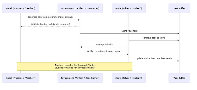
The authors first build a dataset of 500 reasoning tasks across 10 categories such as math logic, spatial reasoning, causal reasoning, and probabilistic reasoning, generated with Claude 3.5 Sonnet, and then collect long reasoning chains from DeepSeek-R1-Distill models with greedy decoding and up to 1000 tokens per answer. They use GPT-4o to label spans in each chain with six tags: initializing, deduction, adding-knowledge, example-testing, uncertainty-estimation, and backtracking, sometimes splitting a sentence into several labeled pieces.
For each behavior and each transformer layer, they gather residual stream activations on tokens in spans with that behavior (plus the token just before the span), define a positive set of prompts that contain the behavior and a negative set as the full dataset, and compute a Difference-of-Means vector between these sets. They then rescale each candidate vector to have the same norm as the mean activation at that layer so that steering strength is comparable across behaviors and layers.
To find where the model actually uses these features, they apply an attribution patching style analysis: they approximate the effect on next-token KL divergence of adding the candidate vector at behavior tokens, and then average this effect across all examples. Plotting this per layer, they see clear peaks in middle layers for each behavior, while early layers have high overlap with token embeddings and so mostly encode lexical identity rather than reasoning behavior; they drop those early layers and select, for each behavior and model, the mid-layer with the largest causal score as the steering site.arxiv
At inference time, they steer by adding or subtracting the chosen vector at that layer at the relevant positions. On 50 new tasks, pushing the vector (positive steering) reliably increases the share of sentences labeled with the target behavior, while pulling it (negative steering) reduces that share, for backtracking, uncertainty, example-testing, and adding-knowledge. They show qualitative traces where more backtracking leads the model to abandon lines of thought and try new ones, while less backtracking makes it stay committed even when wrong. Cosine similarity studies suggest that most behavior vectors are fairly distinct, though uncertainty and backtracking directions are moderately aligned, matching the idea that the model often expresses doubt before switching approaches.
The main message is that these “thinking” behaviors in DeepSeek-R1-Distill are not just vague global traits but can be localized as steerable directions in activation space, giving a light-weight way to dial up or down aspects of reasoning style without retraining. The work is limited by noisy automatic labels, by focusing only on DeepSeek-R1 distills, and by leaving open whether similar mechanisms appear in other reasoning-tuned or RL-only models such as QwQ, but it offers a practical recipe and evidence that fine-grained reasoning control via activation steering is feasible.
Analysis: Reasoning steering is practical today at small-to-medium scale and in research settings, but is not yet a plug‑and‑play industry tool for production systems. It works reliably on specific models and behaviors (like DeepSeek-R1 distills and backtracking/uncertainty), but there are sharp engineering, robustness, and evaluation challenges that slow broader adoption.
In terms of practicality, the core operations—logging residual activations, computing Difference‑of‑Means vectors, and adding them at inference—are straightforward once you have: model weights, hooks into the residual stream, and a labeled dataset of behaviors. The R1 steering paper shows that with 500 tasks and automatic GPT‑4o labeling they can extract behavior vectors and steer backtracking/uncertainty/example‑testing with clear effect sizes across three architectures (Qwen‑1.5B, Qwen‑14B, Llama‑8B). Representation engineering and activation addition papers similarly report that simple linear vectors often suffice to change style, safety, or reasoning behaviors without fine‑tuning. In practice, this makes steering viable for labs that already run open models with custom inference stacks and can accept some extra forward/backward passes during analysis.
However, several reasons explain why this is not widely adopted in mainstream LLM products. First, infrastructure: most commercial inference stacks are optimized for pure forward passes and do not expose an easy or efficient way to hook and modify residuals token‑by‑token, especially at scale and on MoE/quantized kernels. Activation engineering is often described as “interesting but not yet scalable” for production inference. Second, generalization and brittleness: the R1 paper itself limits claims to selected reasoning behaviors on DeepSeek‑R1-Distill; it explicitly notes uncertainty in how results transfer to other models like QwQ or different RL‑trained reasoners. Many activation‑steering results show strong effects on curated benchmarks but less is known about behavior under distribution shift, long contexts, tool use, or adversarial prompts. Third, safety and product risk: steering can create subtle, hard‑to‑predict couplings (e.g., making the model more “uncertain” may alter refusal, verbosity, or calibration), and product teams usually prefer coarse, better‑understood levers (fine‑tuning, system prompts, decoding) that integrate cleanly with existing evals. Finally, developer ergonomics: designing, validating, and monitoring steering vectors requires interpretability and infra expertise; it is not yet a one‑line config option in popular serving stacks. lesswrong, representation engineering
The R1 steering paper and related work use several techniques to verify that steering is real and not just noise or prompt‑artifact. First, they use attribution patching as a causal test: for each candidate vector and layer, they estimate how much adding that vector changes the next‑token logit distribution via a KL‑based metric; layers with larger effects are taken as causally relevant, and they avoid early layers that correlate strongly with embeddings. Second, they run held‑out evaluations: after picking final behavior vectors and layers, they apply positive and negative steering on 50 unseen tasks and quantify changes in the fraction of sentences labeled as backtracking, uncertainty, example‑testing, or adding‑knowledge by an external annotator model (GPT‑4o). Positive steering increases the targeted behavior fraction; negative steering reduces it, with consistent trends across all three DeepSeek‑R1-Distill models. Third, they check representation geometry: cosine similarity matrices show that different behaviors mostly correspond to distinct directions (with moderate correlation between uncertainty and backtracking), supporting the claim that these are separate mechanisms rather than one generic “thinking” axis. Related representation‑engineering work also compares steered vs. unsteered models on downstream metrics (truthfulness, refusal rate, task score) and often measures KL divergence to ensure capability loss is limited. neelnanda, attribution patching
Several ablations or robustness checks appear across this line of work. In the R1 paper, they vary the layer index and use attribution scores as an “ablation over layers,” effectively showing that removing or modifying the vector at different layers changes the KL impact and identifying mid‑layers as critical for reasoning behaviors. They also evaluate the same behaviors on multiple DeepSeek‑R1-Distill sizes and backbones, which functions as an architectural ablation: similar steering effects across Qwen and Llama distills suggest the phenomenon is not a quirk of one model. In broader steering literature, ablations include: comparing simple Difference‑of‑Means vs. more advanced constructions like Contrastive Activation Addition; toggling steering only at certain positions (e.g., only at reasoning tokens vs. all tokens); mean‑centering vs. not; and scaling the vector magnitude to check monotonicity and detect regimes where steering starts to damage core accuracy. Some papers also run safety‑style ablations: does a refusal vector change helpfulness on benign queries, or does a truthfulness vector degrade performance on standard tasks.
Reasoning steering is already practically usable for research, bespoke agents, and specialized deployments where you control the stack and can afford custom hooks and extra evals. It is not yet widely deployed because the infra and methodology are still bespoke, robustness and transfer are incompletely understood, and product teams need standardized evaluations and safety guarantees that are only starting to emerge from this kind of work.
https://www.neelnanda.io/mechanistic-interpretability/attribution-patching